🚧 This training platform and the entire content is under ⚠️construction⚠️ and may not be shared or published! 🚧

Task 2 - Access healthcare - avoid areas

For the main area of Kutupalong Refugee Camp, we have the boundary, the path and road network, water streams and health facilities. In this task we will compare openrouteservice isochrone and QGIS built-in service area catchments. Also we will showcase the avoid area feature in openrouteservice to account for a simple simulated flooding.

Download all datasets here. Save the folder on your computer. Unzip the .zip file. The unzipped folder is structured according to the recommended folder structure for QGIS projects. Under “data > input” you find the geopackage file task2.gpkg which contains the following vector layers:

• camp18_healthcare (points): Healthcare facility locations within camp 18 (from OpenStreetMap)

• camp18_ways (points): Roads and paths within camp 18 (from OpenStreetMap)

• camp18_streams (points): Water streams within camp 18 (from OpenStreetMap)

• camp18_boundary (polygons): The camps legal boundary (from HDX)

STEP 1: Healthcare catchment - Isochrones

First we need to reproject our layers. To do so, open the Processing Toolbox and search for Reproject layer. Select one of your layers as your input layer and choose WGS 84 / UTM zone 46N as your target CRS. Maybe you have to click on the planet button on the right and search for it, if it is not in the list. Leave all other settings at default. Repeat the process with all your layers to reproject all of them.

To get the isochrones click in the toolbar on the ORS Tools plugin Icon. Click on Batch Jobs -> Isochrones from Layer. Leave all settings at default except:

Travel mode	foot-walking
Input Point layer	camp_healthcare
Comma separated ranges	5, 10

Watch here:

STEP 2: Healthcare catchment - QGIS Service area

Isochrones in QGIS can be generated via the service area tool in combination with the minimum bounding geometry tool. Based on a road network, we define origins, a default speed, and a maximum cost.

Open the Processing Toolbox and scroll down to Network Analysis, choose Service area (from layer) or enter “Service area (from layer)” in the search bar. Leave all settings at default except:

Vector layer representing network	camp_ways
Path type to calculate	shortest
Vector layer with start points	camp_healthcare
Travel cost	500 (meters)
Advanced Parameters
Default speed	5.0 (pedestrian)
Topology tolerance	50.0

QGIS on-the-fly creates a network graph from the road and path network. The graph is rather simple. All edges can be traveled in both ways, there are no weights included. Travel cost is represented by the length of a segment and the default average speed. The output is a simplification of the input road & path geometry but with the attributes of the healthcare facilities. For every healthcare facility we see a multiline geometry object in the output. We can style it according to the attribute “@osmId” to see which segments are assigned to which facility.

Question

Can you already spot areas that are not reachable within 500 meters by foot considering the ways?

Your result should look like this:

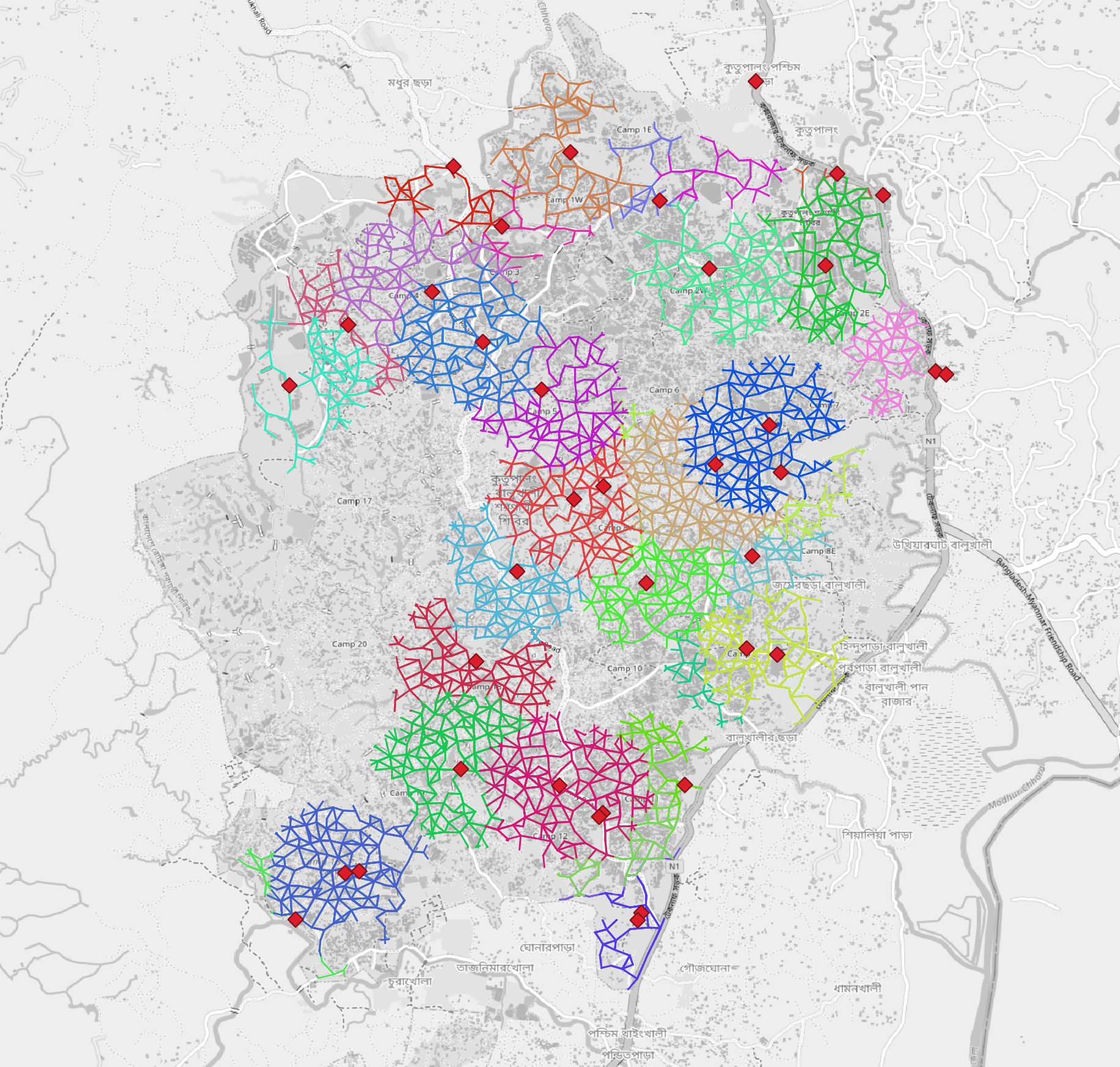
Fig. 223 Network representation of paths within camp18. The color symbolizes groups of ways that are within 500m of the next healthcare facility.

STEP 3: Service area by minimum bounding box

In order to better compare the result of the service areas and isochrones we will again compute the minimum bounding geometry. But this time for the multiline output of the service area tool.

Open the Processing Toolbox, choose Network Analysis,then choose Minimum Bounding Geometryor enter “Minimum Bounding Geometry” in the search bar. Leave all settings at default except:

Input layer	Service area (lines)
Field	@osmId
Geometry type	Convex Hull

Watch here:

Question

Compare the results of both catchments. What differences can you spot?

STEP 4: Healthcare catchment - Isochrones avoid flood

In this part we will again calculate catchments based on the same configured isochrones. But we will include a polygon for the avoid area functionality in openrouteservice. For the avoid area we will use the water streams that run through the main camp area. The avoid areas function of openrouteservice only allows polygons as input, not line geometries. Therefore we need to conduct some preprocessing steps:

1. Reproject the the camp_stream layer to be able to use a metric distanz to buffer. Like before use WGS 84 / UTM zone 46N as the target projection.

2. Now buffer the reprojected stream layer into a polygon layer with a distance of 2 meters

3. We are set to use the buffered stream layer as avoid area or exclusion layer for the routing.

Click in the toolbar on the ORS Tools plugin Icon . Click on Batch Jobs -> Isochrones from Layer. Leave all settings at default except:

Travel mode	foot-walking
Input Point layer	camp_healthcare
Comma separated ranges	5, 10
Advanced Parameters
Polygons to avoid	stream_buffer

Watch here:

Question

Compare the output of the flooded isochrones with the isochrones from before. What differences are apparent for you?