Georeferencing

Georeferencing in QGIS is the process of aligning a raster image, such as a scanned map or aerial photograph, to a known coordinate system so that it can be used in spatial analysis. This involves assigning real-world coordinates to the image by identifying control points on the raster that correspond to known locations on the earth, often using existing vector layers or coordinate grids as a reference.

In many cases, governmental institutions publish maps only as PDFs, without public access to the underlying data. In these cases, knowing how to correctly georeference a map allows you to access and use the information in your GIS analyses. In the case discussed in this chapter, the soil degradation map of Somalia is only available in a PDF report. In order to use the information in a GIS analysis, we can use the georeferencer to assign geographic coordinates to the pixels of the image. After georeferencing the image, the result is a raster file (.tiff). This dataset can be vectorized (converted into vector data) or joined with other raster data, to gain additional information.

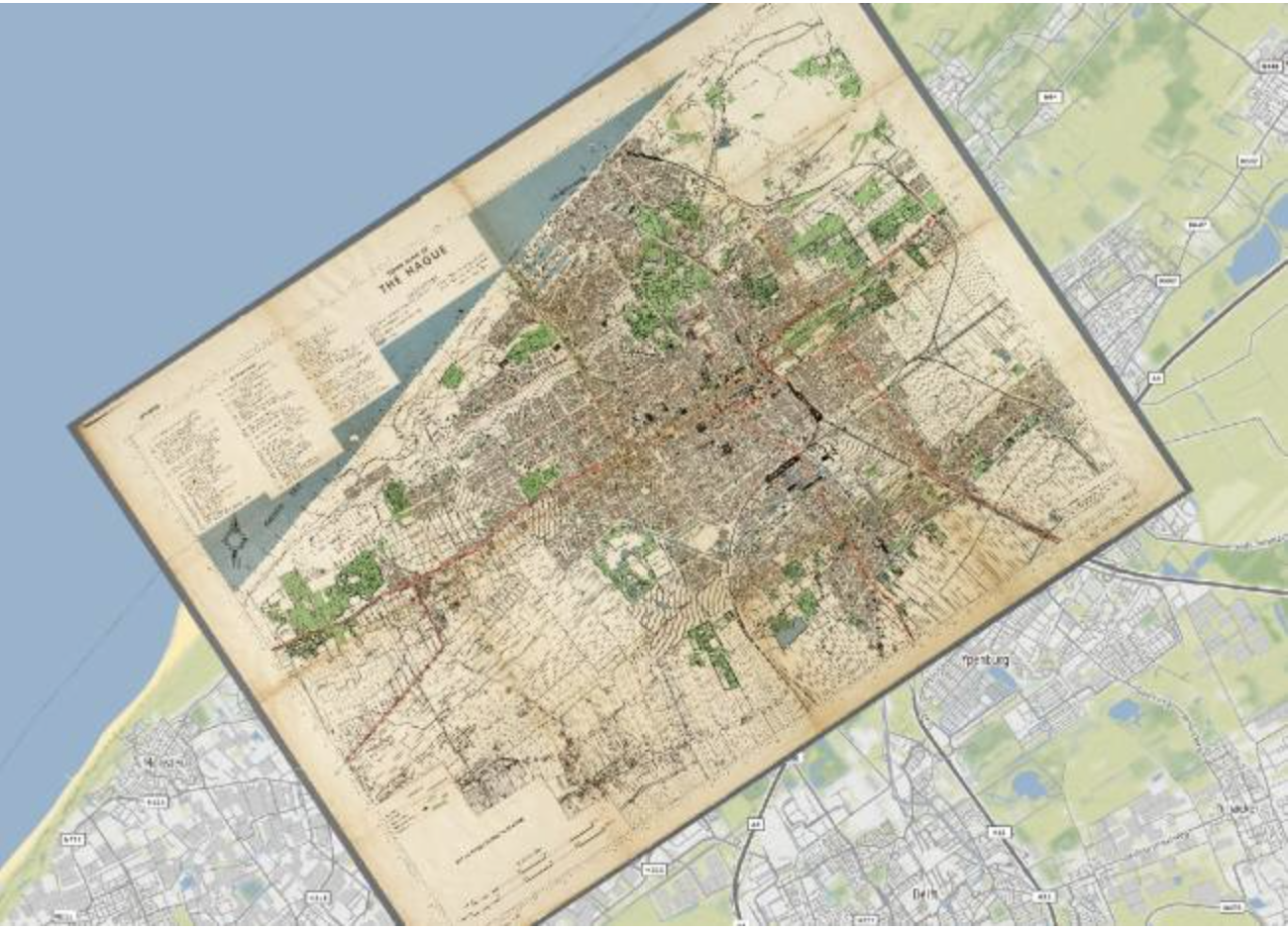
Fig. 70 A digitised old map of the Hague (Source: Kokoalberti)

Georeferencing in QGIS

In QGIS, the Georeferencer tool is used for this process. T Users manually place control points on the raster image and and assigning them a geographic coordinate, either by enter the coordinates manually, or selecting the corresponding point in the QGIS map canvas. These points serve as reference points for the georeferencing algorithm to add geographic coordinates to each pixel in the raster. The algorithm then transforms the image, adjusting its scale, rotation, and position to accurately overlay it with other geospatial layers. Georeferenced images become valuable for digitizing features and conducting spatial analyses within a GIS.

There are several transformation algorithms available in QGIS to gereference a map. If the map is in the same CRS and only needs to be rotated, a linear transformation is sufficient. However, if the image or map is in a different CRS or is visibly skewed, a polynomial transformation is needed. The more complex the transformation algorithm is, the more Ground Control points you need.

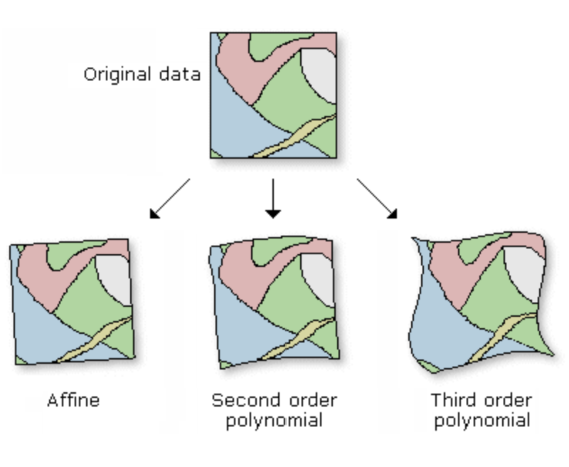
Fig. 71 Different transformation types: linear (left), polynomial 2nd degree (middle), polyonmial 3rd degree (right) (Source: ESRI)

In most cases, you will use either linear, or polynomial (2nd or 3rd degree) transformations. There are many more transformation types to be used in QGIS. Each works best for a specific use case. For an explanation of each transformation type, check out the QGIS Documentation

How to Georeference in QGIS

In order to georeference a PDF map, you need to follow the following steps:

1. Prepare the map you want to georeference either by exporting the relevant page on the PDF or taking a screenshot.

2. In your QGIS window, add a basemap using the XYZ-tiles:

   1. Layer > Add Layer > Add XYZ Tiles.

   2. A new window will open. Under XYZ Connection at the top of the window, select “OpenStreetMap”

   3. Click Add. Ideally, use a basemap where you can identify exact locations on both the basemap and the map you want to georeference.

3. Open the Georeferencer by navigating to the Top Bar > Layer > Georeferencer (see Fig. 72)

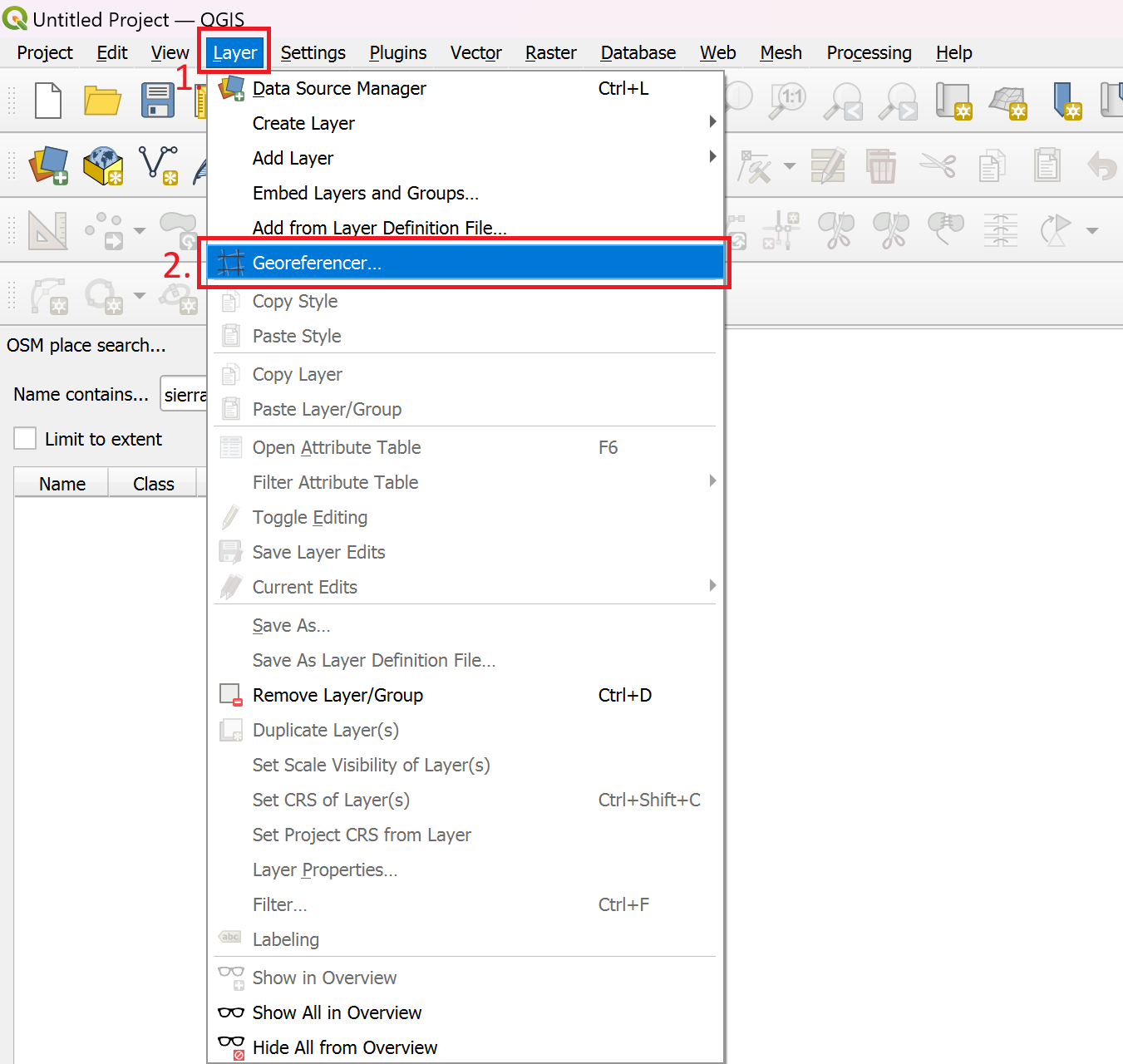
Fig. 72 Opening the Georeferencer in QGIS 3.36

4. A new window will open. This is the georeferencer. To add an image to georeference, click on Open Raster.

5. Select the image of the map you want to georeference. You can load image files, as well as PDFClick Open.

6. The image will appear in the middle of the georeferencer window. Click on Transformation settings....

7. A new window will open. Here you can set the transformation type and the target CRS. Below, you can set the name and save location of the file. Make sure that the Load in project when done is checked.

Note

Setting the appropriate Coordinate Reference System Ideally, you want to set the CRS of the georeferenced map to the same as your project/the other layers in your project. To learn how to choose an appropriate CRS, check out the chapter on projections in module 1.

Note

In most cases, you can leave the transformation type on linear. Regional maps are usually in a conformal projection (i.e. the angles are preserved). Satellite imagery as well. If you realise that the angles are not true, or the map is deformed or distorted, you may need to choose polynomial as transformation type. Polynomial transformations need more Ground Control Points and the points need to be distributed evenly across the map.

8. Click on Ok.

9. Once you have set the transformation type, you can start adding Ground Control Points (GCP) by clicking on Add Point. Ground Control Points are points that you ascribe specific geographic coordinates.

10. Click on a point on the map image. This will be the precise location that you can identify on both the basemap and the map you wish you georeference.

11. Once you clicked on a position, a new window will appear. Here, you add the coordinates to the point you selected. There are two options to do this:

    • Enter the coordinates manually. You will need to know the exact coordinate. Sometimes, you have a coordinate grid on maps where you can

    • Select the points . This mode will minimize the georeferencer and open the QGIS Map canvas. Zoom to the same location you selected on the non-georeferenced map and Click once.

    • Once the coordinates are entered, click Ok

12. The georeferencer window will open again. This time, below the map image, you can see a point in the table. These are the Ground Control Points. Continue adding more GCP. Spread them out over the entire map. Make sure that the Mean error in the bottom right corner of the georeferencer window is as low as possible (below 5 is ideal).

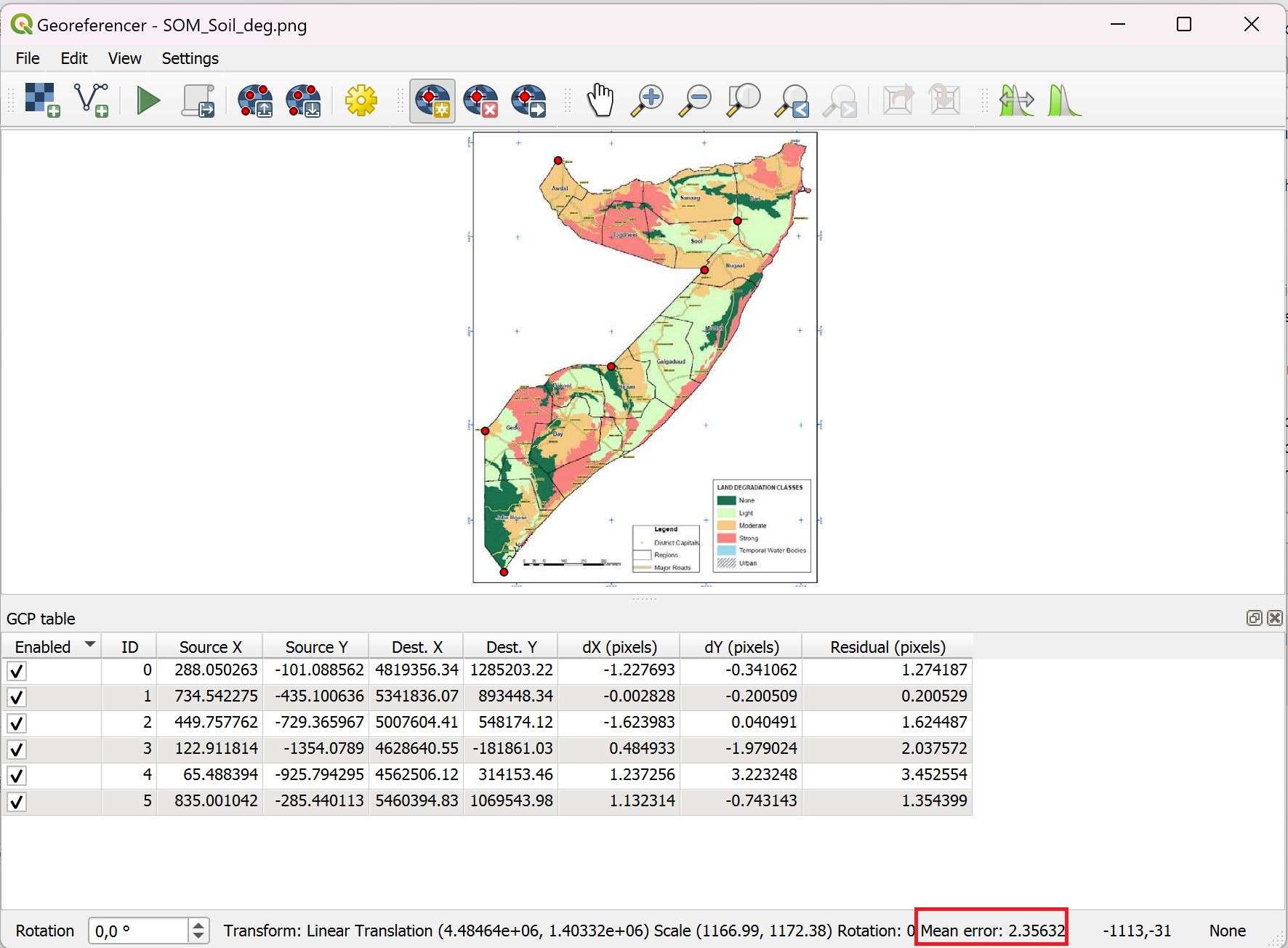
Fig. 73 Georeferencer dialogue in QGIS 3.36

13. Once you have added enough points, click on Start Georeferencing. QGIS will use the Points you added to transform the image into a georeferenced image, where every pixel has GPS coordinates ascribed to it.

14. You can close the georefencer window. Decide wether you want to save the GPC points in a file. If you are not sure if your georeferencing accuracy was precise enough, save the GPC points so you don’t have to do all the work again.

15. Congratulations, the georeferenced map will now appear as a raster layer in your QGIS-project

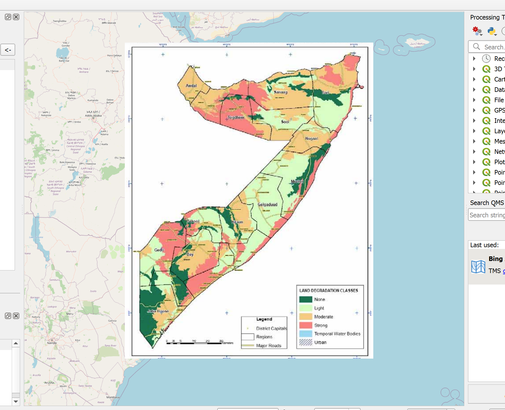
Fig. 74 A georeferenced map of Somalia in the QGIS Map Canvas

Adjusting the georeferenced layer

It is possible to adjust the transparency of the georeferenced map so you can see the underlying layers:

1. Open the Layer Properties by Right-Clicking on the layer and selecting Properties

2. Navigate to the Transparency Tab.

3. Set the global opacity to 50%.

Alternatively, it is also possible to remove the white background. This is done by assigning the white pixels to the Aplha value in the transparency tab under “Custom Transparency Options”.

1. Open the Layer Properties by Right-Clicking on the layer and selecting Properties

2. Navigate to the Transparency Tab.

3. In the Custom Transparency Options box, under Transparency Band, select Band 4 (Alpha).

4. To the right, click on Add value from display

5. Click on the white colour on the georeferenced map in the map canvas.

6. Click Apply.