QGIS Trigger Workflow for Somalia #
Attention
Due to the changes in the availability of FEWSNET data, we are using IPC food insecurity classification instead of the FEWSNET classification. We are currently updating the documentation for the updated trigger model.
The QGIS workflow presented in this article was developed in the framework of the Forecast-based-Action (FbF) Project of the Somalia Red Cresent Society (SRCS), the German Red Cross (GRC) and the Heidelberg Institute for Geoinformation Technology (HeiGIT).
The workflow consists of 15 steps of which 9 are automated in the form of a QGIS Model. In this article, we explain how all 15 steps can be done manually. In practice one needs to do only 6 steps manually, the rest is done by the QGSI Model. The chapter Workflow Automated explains the process and how it is intended in practice. The chapter Workflow Manually is to understand what happens inside of the QGIS Model.
Background #
Setting triggers is one of the cornerstones of the Forecast-based Financing system. For a National Society to have access to automatically released funding for their early actions, their Early Action Protocol needs to clearly define where and when funds will be allocated, and assistance will be provided. In FbF, this is decided according to specific threshold values, so-called triggers, based on weather and climate forecasts, which are defined for each region (see FbF Manual).
For the development of the Somaliland-Somalia Drought Trigger mechanism various datasources were thoroughly analysed. Finally, the main parameters chosen for the trigger based on the historical impact assessment are the twelve month Standard Precipitation Index (SPI12) and the IPC acute food insecurity classification. The exact data used are the documented and forecasted SPI12 (source: ICPAC) and the forecasted IPC classification (8 month forecast, source: FEWSNET), that is used to calculate a population weighted index of food insecurity. The trigger thresholds for both components were optimised towards the most favourable proportion of hit rate and false alarm rate. The emerging thresholds were <-1 for the SPI12 and >=0,7 for the IPC based index. The triggering is done on district level and per district just one trigger initiation per year is possible.
Trigger Statement #
When ICPAC issues a SPI-12 forecast of less than -1 for a district AND the current IPC food insecurity projection reaches at least 0.7 in its derived population weighted index in the same district, then we will act in this district. We expect the lead-time to be 90 days.
Trigger Input Data #
For the trigger mechanism to work properly we currently use different datasets: data that we assume to be fixed in the near term, and variable data which describe the datasets that will be checked for triggering on a monthly base.
Fixed Data #
By fixed data we mean datasets that are needed for the trigger to work, that will most probably not change in the near term. In the long term these datasets can be adapted easily.
Dataset |
Source |
Description |
|---|---|---|
Administrative boundaries |
The administrative boundaries on level 0-2 for Somalia and Somaliland can be accessed via HDX. For this trigger mechanism we provide the administrative boundaries on level 2 (district level) as a shapefile. |
|
Population Counts |
The worldpop dataset in |
Monitoring Data #
Attention
The dataset used for monitoring the food insecurity phase has been updated to the classification and forecast published by the Integrated Food Security Phase Classification as of March 2025. Prior to this, the food insecurity forecast published by FEWSNET had been used.
The drought trigger mechanism is based on two variable monitoring datasets updated monthly: The SPI-12 forecast produced by ICPAC and the Food Insecurity projection produced by FEWSNET. The SPI-12 is used to capture hazard forecasts while the Food Insecurity Projection captures the dynamic vulnerability. In this way upcoming drought events (SPI) that most probably will lead to food insecurity (IPC) will be captured.
What is the Standarized Precipitation Index (SPI-12)? #
The Standardized Precipitation Index (SPI) is a widely used index to characterize meteorological drought. The Standardized Precipitation Index (SPI-12) compares the total rainfall received at a particular location during the last 12 months with the long-term rainfall mean (42 years) for the same period of time at that location.
What is IPC Food Security Projection Data? #
The IPC is a commonly accepted measure and classification to describe the current and anticipated severity of acute food insecurity. The classification is based on a convergence of available data and evidence, including indicators related to food consumption, livelihoods, malnutrition and mortality. Food Insecurity is one of the prioritized impacts of droughts in Somalia which is why it is also used for the triggering mechanism, in a population-weighted index.
Colour |
Phase |
Descriptions |
|---|---|---|
|
1. Minimal |
Households are able to meet essential food and non-food needs without engaging in atypical and unsustainable strategies to access food and income. |
|
2. Stressed |
Households have minimally adequate food consumption but are unable to afford some essential non-food expenditures without engaging in stress-coping strategies. |
|
3. Crisis |
Households either have food consumption gaps that are reflected by high or above-usual acute malnutrition OR are marginally able to meet minimum food needs but only by depleting essential livelihood assets or through crisis-coping strategies. |
|
4. Emergency |
Households either have large food consumption gaps which are reflected in very high acute malnutrition and excess mortality; OR are able to mitigate large food consumption gaps but only by employing emergency livelihood strategies and asset liquidation. |
|
5. Famine |
Households have an extreme lack of food and/or other basic needs even after full employment of coping strategies. Starvation, death, destitution, and extremely critical acute malnutrition levels are evident. (For Famine Classification, area needs to have extreme critical levels of acute malnutrition and mortality.) |


IPC Food Security Projection: #
Three times a year (February, June, and October) FEWSNET estimates most likely IPC classes for the upcoming 8 month (near-term and mid-term projection), available from 2019-current. The near-term projection is called ML1 and is a projection for the upcoming 4 month, the mid-term projection is called ML2 and projects the IPC classes for the 4 subsequent months. For the triggering ML1 (near-term) as well as ML2 (mid-term) projections will be considered.
UPDATE: IPC Classification Data
The food security classification projections are generally published twice a year and usually includes a projection for a period of three months and a current phase, which also spans three months. Due to the unavailability of FEWSNET projections, the trigger model is using the IPC data
Outlook updates are produced almost every month and are also taken into account.
IPC-Population Weighted Index #
To better operationalise the IPC data a simple population-weighted index was developed. Relative population numbers are weighted based on the respective IPC class they falling, in order to give the amount of people in a certain IPC class the importance instead of the IPC class only. Furthermore, population located in a higher IPC class is more important than population located in a lower class. The index is calculated as follows:
\( IPC\ Index = Weights \times \frac{District\ Pop\ per\ IPC\ Phase}{Total\ District\ Pop}\)
Where the weights are defined as:
IPC Phase |
Weight |
|---|---|
IPC 1 |
0 |
IPC 2 |
0 |
IPC 3 |
1 |
IPC 4 |
3 |
IPC 5 |
6 |
The IPC Index represents low-population districts equal to high-population districts. No under-representation of high food insecurity of small districts occurs.
Trigger Workflow Automated #
As explained in the beginning of this chapter, the 9 main steps of the developed trigger workflow are done automatically by a QGIS model. In the previous chapters you have learned the purpose and needed tools of each step and how to perform them manually. In this chapter it is explained how to run the automated model.
The QGIS Model Designer is a visual tool that allows users to create and edit a workflow with all tools available in QGIS that can be used repeatedly in a simple and time-efficient manner. It provides a graphical interface to build workflows by connecting geoprocessing tools and algorithms. The user can define inputs, outputs, and the flow of data between different processing steps.
Troubleshooting the model
When updating the monitoring, make sure you compare the new input layers with the previous input layers. It can happen that the data structure from FEWSNET or ICPAC changes. For example, the attribute columns are called differently, or the values for the classes change. In these cases, the model can break and output error messages.
To fix these issues, take a look at the subsection on Troubleshooting the model.
Step 1: Setting up folder structure #
Purpose: In this step we set up the correct folder structure to make the analysis easier and to ensure consistent results.
Tool: No special tools or programs are needed
Instruction |
Folder Structure |
|---|---|
|

|
The Video below shows the process for setting up the folder for december 2023.
Video: Setting up folder structure
Step 2: Download of the forecast data #
Tool: FileZilla and Internet Browser
The current plans provide that ICPAC will monthly provide the SPI-12 forecast whereas the IPC data will be pulled from the FEWSNET website. FEWS NET publishes IPC data on its website. The main data publications plus the updates of the IPC data amount to the publication of new data almost monthly.
SPI-12 Data #
ICPAC will provide the SPI-12 forecasts on their FTP (File Transfer Protocol). There are different ways to access the FTP-Server. We recommend to install and once set up FileZilla. This will make your work easily repeatable on a monthly basis.
Download Filezilla here.
Install the
.exefile you have downloadedOpen FileZilla
Establish a connection to the FTP Server by inserting the credentials you have been passed (Host, Username and Password) and clicking
Quickconnect.
In FileZilla you have four windows. On the left hand side you will see the folder on your computer in the upper window. By clicking on a folder, the documents in the folder will be shown in the lower left window. On the right hand side, you will see in the upper window the FTP data folder and by clicking on it, the data will be shown in the lower right window.
In order to pass the data from the FTP Server to your own machine you can simply drag and drop the folder or data from the right hand side windows (FTP-Server) to the left hand side windows (your Computer). To do so, firstly navigate to your folder where you need the latest SPI-12 data to be located .../FbF_Drought_Monitoring_Trigger/Monitoring/Year_Month_template/SPI_12. Then drag and drop the latest SPI-12 into the folder.

IPC Data #
The IPC Projection data is provided and regularly updated on the IPC Website.
To navigate to the latest IPC Projection data on Somalia, navigate to Latest Analyses in the top bar > IPC Analyses > Acute Food Insecurity Classification. Here you look for the latest analysis for Somalia.
Go to the IPC website
In the top bar, navigate to
Latest Analyses>IPC Analyses>Acute Food Insecurity Classification.On the new website, select Somalia as a country and select the newest dataset.
On this website, you will see both a map of the current and the projected IPC phase classifications, as well as some metadata. On the right side of the map, click on the button
Download GIS format. This will download the analysis in a GeoJSON format, containing polygons for the administrative boundaries and IPC phases, as well as points for the IPC phase classification for IDP camps.
Download the GeoJSON file. The filename is composed of the country name, the analysis type, and Year and month of publication. E.g.,
Somalia-Acute Food Insecurity January 2025.geoJSON
Note
In some cases, your operating system (Windows) misidentifies the GeoJSON-file as a .customization-file. This does not change anything and can be loaded into your QGIS-project.
Copy the GeoJSON-file into the input monitoring folder.
Example path:
/FbF_Drought_Monitoring_Trigger/Input_monitoring/Year_Month_template/Somalia-Acute Food Insecurity January 2025.geoJSON
Step 3: Loading data into QGIS #
Purpose: In this step, all the data needed will be loaded into QGIS.
Tool: No specific tools are needed, only QGIS.
Open QGIS and create a new project by clicking on
Project->NewOnce the project is created save the project in the folder you created in Step 1 (e.g. 2022_05). To do that click on
Project->Save asand navigate to the folder. Give the project the same name as the folder you created (e.g. 2022_05). Then clickSaveLoad all input data in QGIS by drag and drop. Click on
Project->Save
From the input monitoring folder you created in step 1:
IPC Phase Classification
SPI-12
From the
Fixed_datafolder:district_pop_som
Regions
risk_assessment.gpkg
WorldPop_som.tif
Result: QGIS project with all necessary data ready to be analysed.
This video shows how to setup the QGIS project for April 2022 and how to import all data into the project.
Video: Loading data into QGIS
Step 4: Load the model in the QGIS Model Designer #
Open the tool under
Processing->Graphical ModelerIn the upper panel click
Model->Open Modeland navigate to your folder “FbF_Drought_Monitoring_Trigger”, mark the “Triggermodel_Somalia.model3” (or the updated model: “IPC_Som_drought_revision_2.1.model3”) file an click onOpen. The model will open and you will see yellow, white and green boxes.
Video: Open Model
Box |
Significance |
Description |
|---|---|---|
Yellow |
Model Input |
Definition of the input data for the model the model will perform on |
White |
Algorithms |
Algorithms or Tools are specific geoprocessing steps that perform specific tasks, such as clipping, reprojecting or buffering. |
Green |
Model Output |
The results created by the model (Output layers) are automatically added to your layers panel in your QGIS project interface |
Step 5: Run the model #
Model Input & Output
Attention
In the dropdown list, only layers that are currently loaded in your QGIS Project will be displayed.
For each of these mandatory inputs, you click on the dropdown arrow and choose the respective file.
In the upper panel click on
Model->Run Model. A window will open where you need to define the model input and output.The model needs the following 3 inputs:
Somalia-Acute Food Insecurity January 2025: IPC ProjectionSPI12(SPI12 forecast): SPI-12 raster dataWorldpop(Population Raster data): Worldpop raster data
Further down, you have to specify where to save the output:
Trigger_activation: Click on the three points ->
-> Save to Fileand navigate toResultsfolder in the folder you created in step 1 (Year_month). Give the output the name:
Trigger_activation
Indices: Click on the three points-> Save to Fileand navigate toResultsfolder in the folder you created in step 1 (Year_month). Give the output the name:
Indices
IPC_Phase_C:Click on the three points-> Save to Fileand navigate toResultsfolder in the folder you created in step 1 (Year_month). Give the output the name:
IPC_Phase_C
IPC_Phase_P:Click on the three points-> Save to Fileand navigate toResultsfolder in the folder you created in step 1 (Year_month). Give the output the name:
IPC_Phase_P
Click
Run. Your results layer will appear in the main QGIS window. You can close the graphical modeller window.
Video: Input and output Model
Step 6: Visualisation of results #
Purpose: Definition of how features are represented visually on the map.
Tool: Symbology tab
Trigger Activation
Right click on the “Trigger_activation” layer ->
Properties->SymbologyIn the down left corner click on
Style->Load StyleIn the new window click on the three points
. Navigate to the “FbF_Drought_Monitoring_Trigger/layer_styles” folder and select the file “Style_Trigger_Activation.qml”.Click
Open. Then click onLoad StyleBack in the “Layer Properties” Window click
ApplyandOK
Info: Trigger Activation Layer
You will now see districts where no trigger is activated in green and districts with trigger activation in pink.
The “Style_Trigger_Activation.qml” style layer is configured to show the district names only where the trigger is actually activated. If there is no trigger activation you can activate the admin 1 boundary layer for better map orientation (see Administrative 2 Boundaries below)

Risk Assessment
Right click on the “risk_assessment_districts” layer ->
Properties->SymbologyIn the down left corner click on
Style->Load StyleIn the new window click on the three points
. Navigate to the “FbF_Drought_Monitoring_Trigger/layer_styles” folder and select the file “somalia_risk_assessment_style.qml” style layer.Move the “risk_assessment_district” layer below “Trigger_Activation” layer (Layer Concept).
Back in the “Layer Properties” Window click
ApplyandOK
Info: Risk Assessment Layer
For the creation of an Intervention Map we will have to add the risk assessment data and the respective style file. For this first of all load from “FbF_Drought_Monitoring_Trigger/Fixed_data/Risk_Assessment” the file “risk_assessment_districts.gpkg”. This file is the output of the conducted risk assessment and contains a risk value for each district of Somaliland and Somalia. In order to visualize it
Administrative 2 Boundaries (Regions)
Right click on the “Som_Admbnda_Adm1_UNDP” (Regiond) layer ->
Properties->SymbologyIn the down left corner click on
Style->Load StyleIn the new window click on the three points
. Navigate to the “FbF_Drought_Monitoring_Trigger/layer_styles” folder and select the file “somalia_risk_assessment_style.qml”.Click
Open. Then click onLoad StyleBack in the “Layer Properties” Window click
ApplyandOKAdd a the OpenStreetMap basemap by clicking on
Layer->Add Layer->Add XYZ layer...-> Select the OpenStreetMap. ClickAdd. (Wiki basemap)Place the OpenStreetMap basemap on the bottom.
Delet all layers exept:
Trigger_activation
risk_assessment_districts
Som_Admbnda_Adm1_UNDP
OpenStreetMap
Video: Visualisation of results
Intervention Map without Trigger activation |
Intervention Map with Trigger activation |
|---|---|
|
|
Attention
Remember the layer concept and make sure the basemap layer is at the bottom of your layers panel.
Step 7: Making the Print Map #
Purpose: Viualisation of the map features in a printable map layout
Tool: Print Layout
If not done before, delet all layers expect Trigger_activation, risk_assessment_districts and OpenStreetMap
Open a new print layout by clicking on
Project->New Print Layout-> enter the name of your current Project e.g “2022_04”.Go the the FbF_Drought_Monitoring_Trigger
folder and drag and drop the fileTrigger_activation_Intervention_map.qpt` in the print layoutChange the date to the current date by clicking on “Further map info…” in the items panel. Click on the
Item Propertiestab and scroll down. Here you can change the date in theMain Propertiesfield.Adjust the Lgend by clicking on the legend in the
Item Propertiestab and scroll down until you see theLegend itemsfield. If it is not there check if you have to open the dropdown. Make sureAuto updateis not checked.Remove all itemes in the legend be clicking on the item and then on the red minus icon below.
Add Trigger_activation and risk_assessment_districts to the legend by clicking on the green plus and click on the layer and click
ok
Video: Making print map
Attention
Make sure you edit the Map Information on the template, e.g. current date. Also make sure to check the legend items: Remove unnecessary items and eventually change the names to meaning descriptions.
In order to easily visualize the output of the trigger analysis we provide you with a map template that can be used as a base for your visualization. You can find the template in the following directory: “…/FbF_Drought_Monitoring_Trigger/maps_somalia_template_risk_assessment.qpt”.
You can also adapt the template to your needs and preferences. You can find help here.
Attention
Make sure you edit the Map Information on the template, e.g. current date. Also make sure to check the legend items: Remove unnecessary items and eventually change the names to meaning descriptions.
Step 8: Exporting the Map #
Purpose: Export the designed and finalized map layout in order tp print it as a pdf or format of your choice.
Tool: Print Layout
When you have finished the design of you map you can export it as pdf or image file in different datafromats.
Export as Image
In the print layout click on
Layer->Export as ImageChose the Result folder in the folder you have created in step 1. Give the file the name of the project e.g 2022_04
Click on
SaveThe window “Image Export Options” will appear. Click
SaveNow the image can be found in the result folder in the folder you created in Step 1
Export as PDF
In the print layout click on
Layer->Export as PDFChose the Result folder in the folder you have created in step 1. Give the file the name of the project e.g 2022_04
Click on
SaveThe window “PDF Export Options” will appear. For the best results, select the
losslessimage compression.Click
SaveNow the image can be found in the result folder in the folder you created in Step 1
Video: Export image and PDF
Troubleshooting the Model #
In some cases, for example when the data structure of the input layers change, the model can break. To make sure that the model functions correctly, follow these troubleshooting steps. In most cases, the problems are happening at the input stage (yellow boxes).
When monitoring the trigger, take a closer look at the new data downloaded from FEWSNET or ICPAC. Are there any changes in the names of the columns or values?
If you get an error message, read the error message. Which input or which step is producing the error?
Take a look at the attribute table of the input layer that is responsible for this layer and at the processing algorithm (white boxes) this layer is feeding into. You can open the parameters for the algorithms by clicking on the
...in the algorithm box. A new window will open with the parameters for the algorithm. What value is the algorithm expecting? What values or data is available in the input layer?Adjust the values the algorithms is expecting or preprocess the input layer so the columns and values are exactly what the algorithm expects.
For example,
FEWSNET changed the structure of the IPC Food Security Projection Data:
The data for ML1 and ML2 is no longer available as two distinct shapefiles, but the (overlapping) polygons for both scenarios are contained in a single geojson file.
Furthermore, the values for the different food insecurity phase (1 to 5: Minimal, Stressed, Crisis, Emergency, Famine) are no longer in a column called “ML1” and “ML2” respectively, but in a column with the name “value”.
The model components “weighing pop-sum based on IPC phase” are expecting a column with the name “ML1” and “ML2”, but the columns with this information (IPC Phase) with the new input layers are no longer called “ML1” and “ML2” and are called “value”.
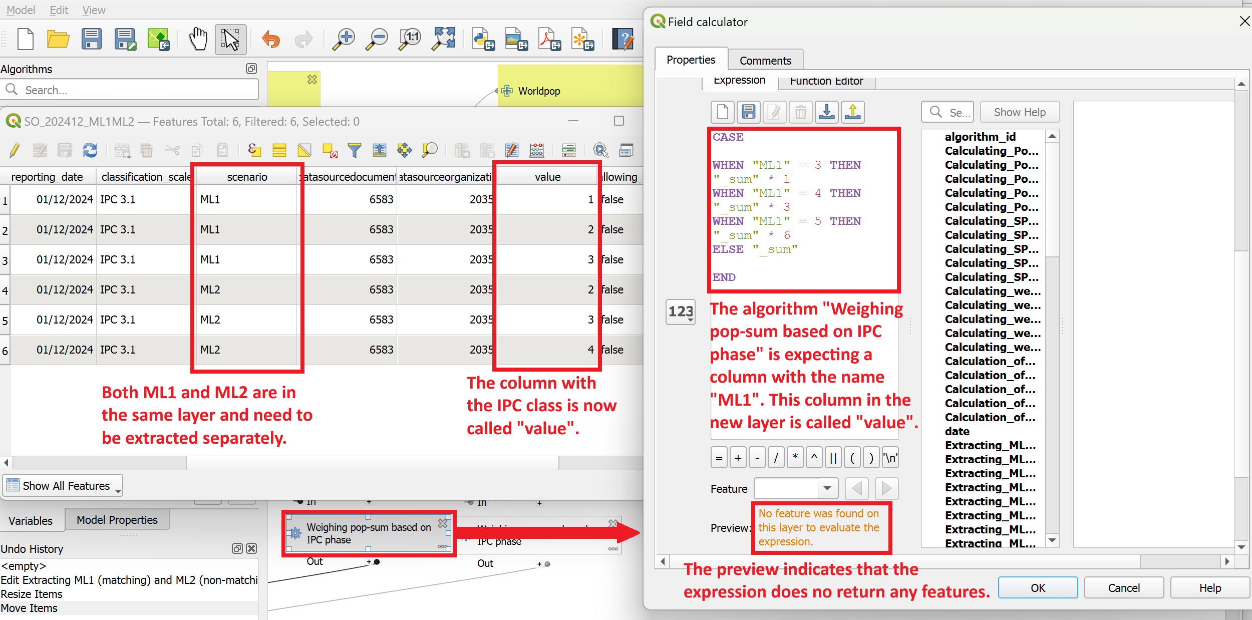
To fix the model, we need to do the following:
Extract the “ML1” and “ML2” polygons as two separate vector layers. We can use the tool “Extract by Attribute”.
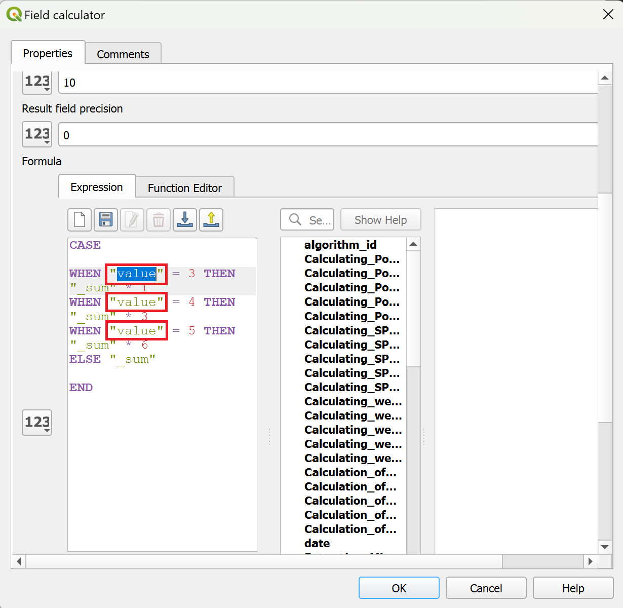
In the field calculator, we need to adjust the expression so it includes the correct column. Change “ML1” and “ML2” into “value” respectively.
Trigger Workflow Manually #
Attention
As of may 2025, the trigger model uses the IPC Phase Classification analysis by the IPC and no longer by FEWSNET. The data format has changed and the manual workflow no longer works as described below. Due to differences in the data structure as well as the extent of the geometries, the manual workflow has changed considerably.
Step 1: Setting up folder structure #
Purpose: In this step we set up the correct folder structure to make the analysis easier and to ensure consitent results.
Tool: No special tools or programs are needed.
Instruction |
Folder Structure |
|---|---|
|
|
The Video below shows the process for setting up the folder for decmber 2023.
Video: Setting up folder structure
Step 2: Download of the forecast data #
Tool: FileZilla and Interent Browser
The current plans provide that ICPAC will monthly provide the SPI-12 forcast whereas the IPC data will be pulled from the FEWSNET website. FEWS NET publishes IPC data on its website. The main data publications plus the updates of the IPC data amount to the publication of new data almost monthly.
SPI-12 Data #
ICPAC will provide the SPI-12 forecasts on their FTP (File Transfer Protocol). There are different ways to access the FTP-Server. We recommend to install and once set up FileZilla. This will make your work easily repeatable on a monthly basis.
Download Filezilla here.
Install the
.exefile you have downloaded.Open FileZilla.
Establish a connection to the FTP Server by insterting the credentials you have been passed (Host, Username and Password) and clicking
Quickconnect.
In FileZilla you have four windows. On the left hand side you will see the folder on your computer in the upper window. By clicking on a folder, the documents in the folder will be shown in the lower left window. On the right hand side, you will see in the upper window the FTP data folder and by clicking on it, the data will be shown in the lower right window.
In order to pass the data from the FTP Server to your own machine you can simply drag and drop the folder or data from the righthandside windows (FTP-Server) to the lefthandside windows (your Computer). To do so, firstly navigate to your folder where you wneed the latest SPI-12 data to be located .../FbF_Drought_Monitoring_Trigger/Monitoring/Year_Month_template/SPI_12. Then drag and drop the latest SPI-12 into the folder.
IPC Data #
The IPC Projection data is provided and regularly updated on the IPC Website.
To navigate to the latest IPC Projection data on Somalia, navigate to Latest Analyses in the top bar > IPC Analyses > Acute Food Insecurity Classification. Here you look for the latest analysis for Somalia.
Go to the IPC website
In the top bar, navigate to
Latest Analyses>IPC Analyses>Acute Food Insecurity Classification.On the new website, select Somalia as a country and select the newest dataset.
On this website, you will see both a map of the current and the projected IPC phase classifications, as well as some metadata. On the right side of the map, click on the button
Download GIS format. This will download the analysis in a GeoJSON format, containing polygons for the administrative boundaries and IPC phases, as well as points for the IPC phase classification for IDP camps.
Download the GeoJSON file. The filename is composed of the country name, the analysis type, and Year and month of publication. E.g.,
Somalia-Acute Food Insecurity January 2025.geoJSON
Note
In some cases, your operating system (Windows) misidentifies the GeoJSON-file as a .customization-file. This does not change anything and can be loaded into your QGIS-project.
Copy the GeoJSON-file into the input monitoring folder.
Example path:
/FbF_Drought_Monitoring_Trigger/Input_monitoring/Year_Month_template/Somalia-Acute Food Insecurity January 2025.geoJSON
Step 3: Loading data into QGIS #
Purpose: In this step, all the data needed will be loaded into QGIS.
Tool: No specific tools are needed, only QGIS.
Open QGIS and create a new project by clicking on
Project->NewOnce the project is created save the project in the folder you created in Step 1 (e.g. 2022_05). To do that click on
Project->Save asand navigate to the folder. Give the project the same name as the folder you created (e.g. 2022_05). Then clickSaveLoad all input data in QGIS by drag and drop. Click on
Project->Save
From the folder you created in step 1
IPC Phase Classification
SPI-12
From the
Fixed_datafolder:district_pop_som
Regions
risk_assessment.gpkg
WorldPop_som.tif
Result: QGIS project with all necessary data ready to be analysed.
This video shows how to setup the QGIS project for April 2022 and how to import all data into the project.
Video: Loading data into QGIS
Step 4: Formatting the ADM2-names #
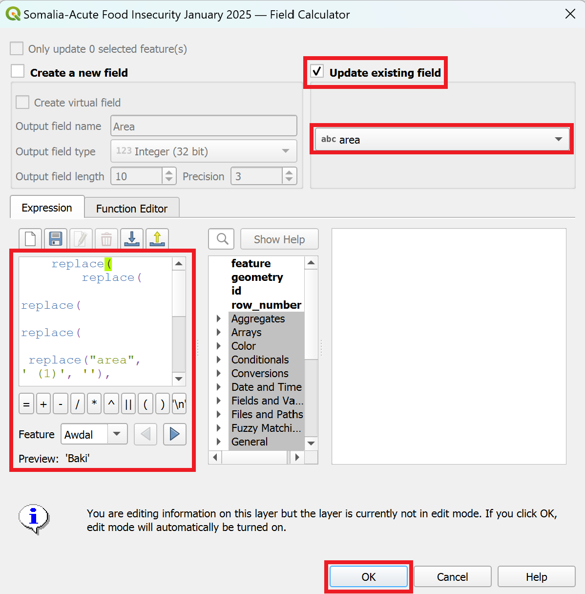
Purpose: The GeoJSON file from IPC contains a polygon layer that contains the administrative boundaries and the IPC phase for the current analysis (C) and the projection (P). However, it is all contained in one layer. To be able to perform our analysis steps, we need to prepare the data. In the column where the adm2-names are saved, there are several polygons with the same adm names, but have a “(1)” or “(2)” added at the end. We need to remove number in the parantheses so we can dissolve the polygons in the next step.
Tool: Field Calculator
Instruction |
Field Calculator |
|---|---|
replace(
    replace(
        replace(
            replace(
                replace("area", ' (1)', ''),
                ' (2)', ''
            ),
            ' (3)', ''
        ),
        ' (4)', ''
    ),
    ' (5)', ''
)
|
|
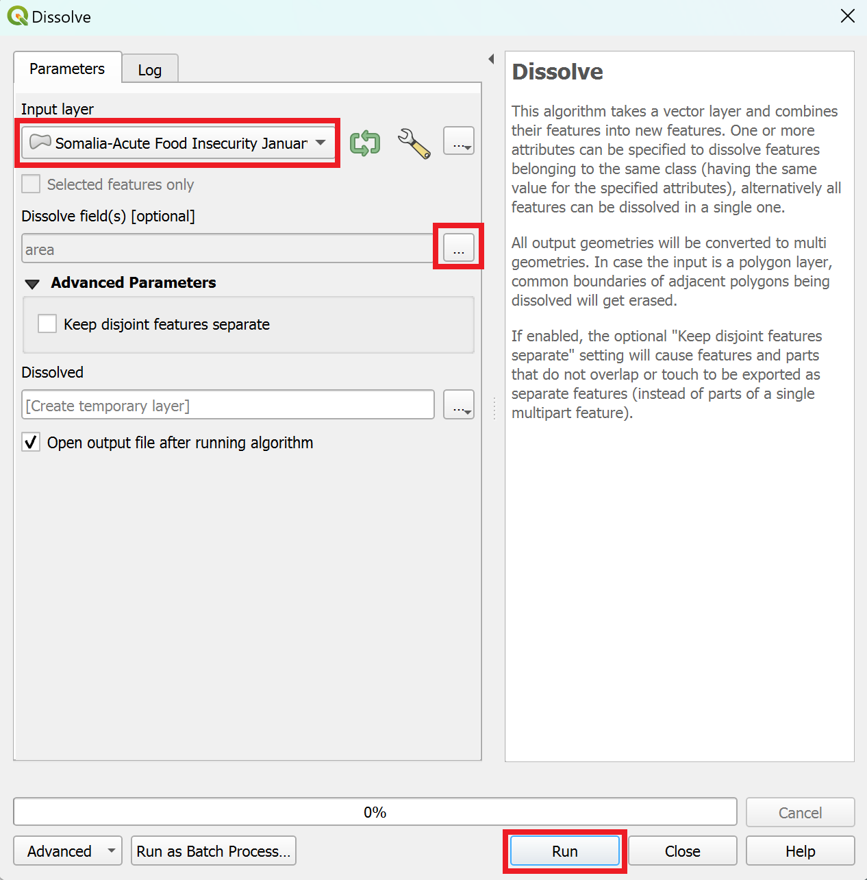
Step 5: Dissolving admin 2 polygons #
Purpose: To get a layer of the administrative boundaries for the district, we need to dissolve the polygons from the formatted layer from the previous step using the field “area”. This will output one polygon per distinct “area” value. In other words a layer withe adm2 boundaries.
Tool: Dissolve
Note
We cannot use a different polygon layer with the adm2 boundaries as we are calculating the population per polygon in the following steps and the polygons need to match exactly in order to get the correct population weighing.
Instruction |
Dissolve |
|---|---|
|
|
Step 6: Add population statistics to the adm2 layer #
Purpose: For the calculation of the IPC index, we need to have the population per adm2 polygon. Using the worldpop raster layer, we can calculate the population inside each district using the output from the previous step
Step 4: Extracting ML1 and ML2 from the GeoJSON layer #
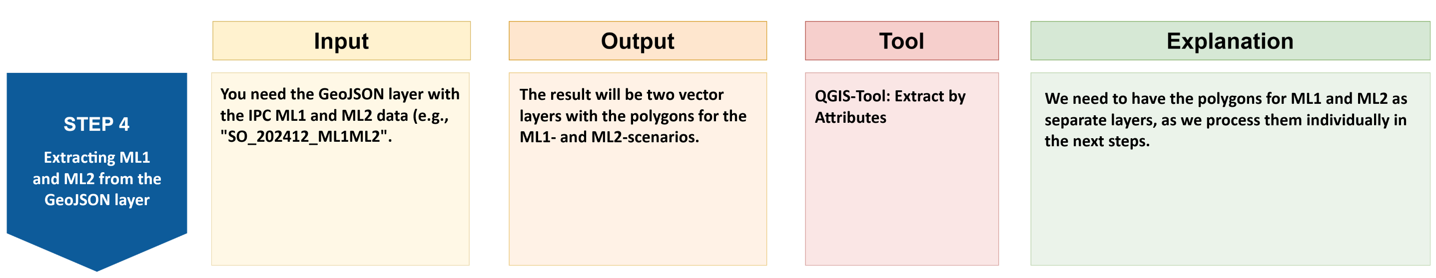
Purpose: The GeoJSON file from FEWSNET with the IPC data contains both the ML1 and ML2 polygons in the same layer. In order to process these polygons separately in the next step, we need to extract and save them as new layers.
Tool: “Extract by Attributes”
Instruction |
Extract by Attribute |
|---|---|
|

|
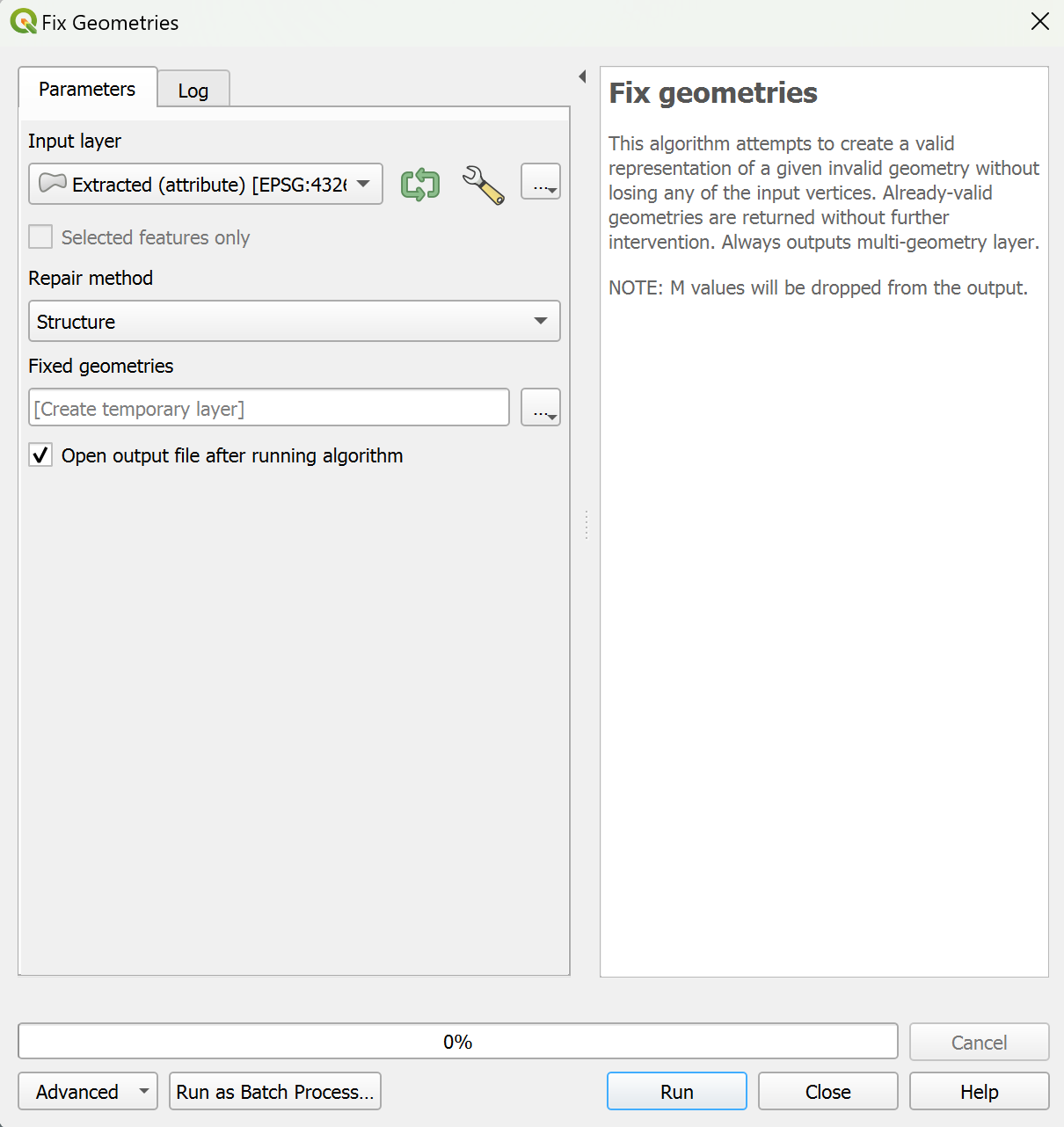
Step 5: Fixing the Geometries for the ML 1 & ML 2 layers #
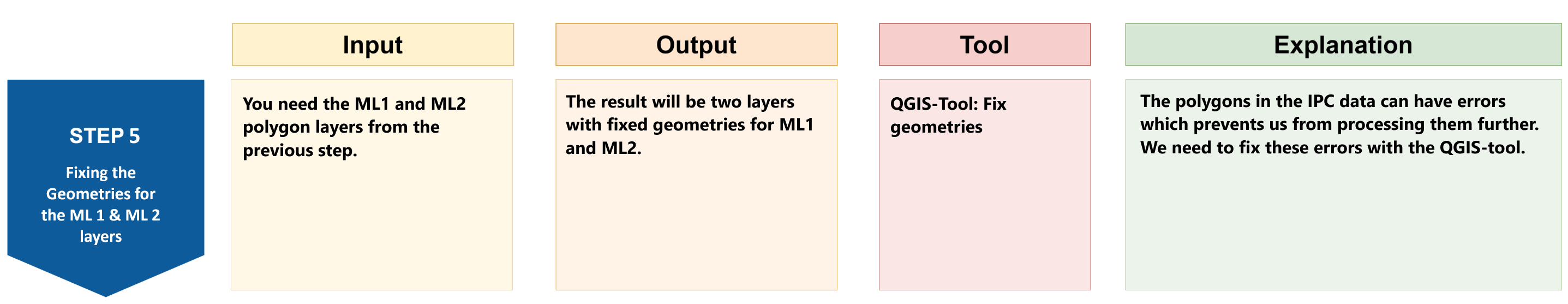
Purpose: The aim is to fix the errors in the geometries of each layer. Otherwise, we would receive error messages in the further steps.
Attention
You need to perform this step two times. One time for ML 1 and a second time for ML 2.
Tool: Fix geometries
Instruction |
Fix geometries |
|---|---|
|
|
Step 6: Intersection of ML 1 & ML 2 data with the district polygons #
Purpose: The goal is to receive polygon layers which share both the borders and the attributes of both input layers.
Attention
You need to perform this step two times. One time for ML 1 and a second time for ML 2.
Tool: Intersection
Instruction |
Intersection |
|---|---|
|
|
Result: After doing this for ML1 and ML2 you should have two polygon layers, each containing all columns of ML1 (or ML2) and district_pop_sum.
Note
The resulting layer can have more rows than the original layers.
The video shows the whole process on the example of ML 1.
Video: Intersection of ML 1 & ML 2 data with the district polygons
Step 7: Calculation of Population per Intersection Polygon #

Purpose: Here we calculate the population in each polygon of the intersection layer from step 4.
Attention
You need to perform this step two times: One time for ML 1 and a second time for ML 2.
Tool: Zonal Statistics
Instruction |
Zonal Statistics |
|---|---|
|
|
Result: The result should be the “ML1_zonal_statistic” and “ML2_zonal_statistic” polygon layers. These layers should have the same columns in the attribute table plus the column “_sum”, which is the number of people living in the single parts of the polygons.
Video: Calculation of Population per Intersection Polygon
Step 8: Weighting of the Population based on IPC-Phase #

Purpose: The purpose of this step is the weighting of the population in the five IPC phases as described in IPC Data.
Attention
You need to perform this step two times. One time for ML 1 and a second time for ML 2.
Tool: Field Calculator
Right-click on the layer “ML1_zonal_statistic” (or “ML2_zonal_statistic”) ->
Open Attribute Table-> click onField Calculator to open the field calculator
Check “Create new field”
Output field name: Name the new column “pop_sum_weighted”Result field type: Decimal number (real)Add the code block from Input into the
Expressionfield and clickok
ML 1 |
ML 2 |
|---|---|
CASE

WHEN "value" = 3 THEN "_sum" * 1
WHEN "value" = 4 THEN "_sum" * 3
WHEN "value" = 5 THEN "_sum" * 6
ELSE "_sum"

END
|
CASE

WHEN "value" = 3 THEN "_sum" * 1
WHEN "value" = 4 THEN "_sum" * 3
WHEN "value" = 5 THEN "_sum" * 6
ELSE "_sum"

END
|
Save the new column by clicking on
 in the attribute table and end the editing mode by clicking on
Here is the Field Calculator window of how it should look to calculate pop_sum_weighted for ML1.
Result: The two layers “ML1_zonal_statistic” and “ML2_zonal_statistic” should now both have the column “pop_sum_weighted”.
The video shows the whole process with the the example of ML 1.
Video: Weighting of the Population based on IPC-Phase
Step 9: Adding the total district population to Intersection Polygons #

Purpose: Now we want to add a column with the total district population to “ML1_zonal_statistic” and “ML2_zonal_statistic”.
Attention
You need to perform this step two times. One time for ML 1 and a second time for ML 2.
Tool: Join attributes by field value
Instruction |
Join attributes by field value |
|---|---|
|

|
Result: Now you should have to new polygon layer named “ML1_join” and ML2_Join” containing the column districtpo.
Video: Adding the total district population to Intersection Polygons
Step 10: Calculation of the Population Proportion per Intersection Polygon #

Purpose: In this step we calculating the IPC-Population Weighted Index for every small part of the polygon layer.
Attention
You need to perform this step two times. One time for ML 1 and a second time for ML 2.
Tool:Field Calculator
Right-click on Intersection_population Polygons layer -> “Attribute Table”-> click on
Field Calculatorto open the field calculatorCheck
Create new fieldOutput field name: Name the new column “Index_per_IPCPolygon_ML1” (or “Index_per_IPCPolygon_ML2”)Result field type: Decimal number (real)Add the code into the
Expressionfield
"pop_sum_weighted"/"districtpo"
Click
okSave the new column by clicking on
in the attribute table and end the editing mode by clicking on
Result: Both layer “ML1_join” and ML2_Join” should now have the column “Index_per_IPCPolygon_ML1” or “Index_per_IPCPolygon_ML2”. The numbers in this column have to be smaller than in the “district” column.
The video shows the whole process with the the example of ML 1.
Video: Calculation of Population Proportion per Intersection Polygon
Step 11: Calculate the IPC Index per District #
Purpose: The purpose of this step is to calculate a population weighted mean over the IPC classes that fall within a district, in order to give the amount of people living in a certain IPC class more importance than just the area affected by a certain IPC class. The result is a IPC Index value for each district.
Tool: Join attribute by location (summary)
Instruction |
Join attribute by location (summary) |
|---|---|
|
|
Result: As a result, your two layers “ML1_join_location” and “ML2_join_location” should have the column “Index_per_IPCPolygon_ML1_mean” or “Index_per_IPCPolygon_ML2_mean”. Furthermore, the number of rows should be the exact number of districts in Somalia and the polygons should have the exact shape of the districts.
Video: Calculate IPC Index per District
Step 12.: Join ML1 and ML2 #

Purpose: The purpose of this step is to merge “ML1_join_location” and “ML2_join_location” into one layer so we have the IPC-Index for all districts.
Tool: Join attributes by field value
Instruction |
Join attribute by location (summary) |
|---|---|
|
|
Result: Layer with the districts of Somalia and the IPC-Index of each district.
Video: Join ML1 and ML2 I
Step 13: Calculation of SPI-12 Mean per District #

Purpose: Calculate the mean value over the SPI-12 values of all pixels that fall within a scertain districts area, in order to have one SPI-12 value for each district.
Tool: Zonal Statistics
Instruction |
Zonal Statistics |
|---|---|
|
|
Result: A layer of all districts of Somalia with the mean SPI-12.
Video: Calculation of SPI12 Mean per District
Step 14: Join SPI-12 Mean to the IPC Index #
Purpose: The purpose of this step is to merge data from two different data sources into one data frame so that it can be jointly analysed.
Tool:Join attributes by field value
Instruction |
Join attributes by field value |
|---|---|
|
|
Result: The result will be a layer of all districts of Somalia with the mean SPI-12 and the IPC-Index of each district.
Video: Join SPI12 Mean to the IPC Index
Step 15: Evaluate the Trigger Activation #
Purpose: The purpose of this step is to gain a quick overview of possible trigger activation without having to revise the actual data. Instead we will have a binary column with trigger = yes or trigger=no values.
Tool: Field Calculator
Right-click on “IPC_index_SPI_12_district” layer ->
Attribute Table-> click onField Calculator to open the field calculatorCheck
Create new fieldOutput field name: Name the new column “Trigger_activation”Result field type: Text (string)Add the code below into the
Expressionfield
Code |
|---|
CASE

WHEN "Index_per_IPCPolygon_ML1_mean" >0.7 AND "Index_per_IPCPolygon_ML2_mean" > 0.7
AND
"SPI12_mean" < -1
THEN 'yes'
ELSE 'no'

END
|
Click
okSave the new column by clicking on
in the attribute table and end the editing mode by clicking on
Result: A layer with all districts of Somalia with a column of “Yes” and “No” values indicating whether the trigger levels have been reached or not.
Video: Evaluate Trigger Activation
Step 16: Visualisation of results #

Purpose: Definition of how features are represented visually on the map.
Tool: Symbology
Trigger Activation
Right cklick on the “Trigger_activation” layer ->
Properties->SymbologyIn the down left corner click on
Style->Load StyleIn the new window click on the three points
. Navigate to the “FbF_Drought_Monitoring_Trigger/layer_styles” folder and select the file “Style_Trigger_Activation.qml”.Click
Open. Then click onLoad StyleBack in the “Layer Properties” Window click
ApplyandOK
Info: Trigger Activation Layer
You will now see districts where no trigger is activated in green and districts with trigger activation in pink.
The “Style_Trigger_Activation.qml” style layer is configured to show the district names only where the trigger is actually activated. If there is no trigger activation you can activate the admin 1 boundary layer for better map orientation (see Administrative 2 Boundaries below)
Risk Assessment
Right click on the “risk_assessment_districts” layer ->
Properties->SymbologyIn the down left corner click on
Style->Load StyleIn the new window click on the three points
. Navigate to the “FbF_Drought_Monitoring_Trigger/layer_styles” folder and select the file “somalia_risk_assessment_style.qml” style layer.Move the “risk_assessment_district” layer below “Trigger_Activation” layer (Layer Concept).
Back in the “Layer Properties” Window click
ApplyandOK
Info: Risk Assessment Layer
For the creation of an Intervention Map we will have to add the risk assessment data and the respective style file. For this first of all load from “FbF_Drought_Monitoring_Trigger/Fixed_data/Risk_Assessment” the file “risk_assessment_districts.gpkg”. This file is the output of the conducted risk assessment and contains a risk value for each district of Simaliland and Somalia. In order to visualize it
Administrative 2 Boundaries (Regions)
Right click on the “Som_Admbnda_Adm1_UNDP” (Regiond) layer ->
Properties->SymbologyIn the lower right corner click on
Style->Load StyleIn the new window, click on the three points
. Navigate to the “FbF_Drought_Monitoring_Trigger/layer_styles” folder and select the file “somalia_risk_assessment_style.qml”.Click
Open. Then click onLoad StyleBack in the “Layer Properties” Window click
ApplyandOKAdd a the OpenStreetMap basemap by clicking on
Layer->Add Layer->Add XYZ layer...-> Select the OpenStreetMap. ClickAdd. (Wiki basemap)Place the OpenStreetMap basemap on the bottom.
Delet all layers exept:
Trigger_activation
risk_assessment_districts
Som_Admbnda_Adm1_UNDP
OpenStreetMap
Video: Visualisation of results
Intervention Map without Trigger activation |
Intervention Map with Trigger activation |
|---|---|
|
|
|
Attention
Remember the layer concept and make sure the basemap layer is at the bottom of your layers panel.
Step 17: Making the print map #

Purpose: Viualization of the map features in a printable map layout
Tool: Print Layout
If not done before, delet all layers expect Trigger_activation, risk_assessment_districts and OpenStreetMap
Open a new print layout by clicking on
Project->New Print Layout-> enter the name of your current Project e.g “2022_04”.Go the the FbF_Drought_Monitoring_Trigger
folder and drag and drop the fileTrigger_activation_Intervention_map.qpt` in the print layoutChange the date to the current date by clicking on “Further map info…” in the items panel. Click on the
Item Propertiestab and scroll down. Here you can change the date in theMain Propertiesfield.Adjust the Lgend by clicking on the legend in the
Item Propertiestab and scroll down until you see theLegend itemsfield. If it is not there check if you have to open the dropdown. Make sureAuto updateis not checked.Remove all itemes in the legend be clicking on the item and then on the red minus icon below.
Add Trigger_activation and risk_assessment_districts to the legend by clicking on the green plus and click on the layer and click
ok
Video: Making print map
Attention
Make sure you edit the Map Information on the template, e.g. current date. Also make sure to check the legend items: Remove unnecessary items and eventually change the names to meaning descriptions.
In order to easily visualize the output of the trigger analysis we provide you with a map template that can be used as a base for your visualization. You can find the template in the following directory: “…/FbF_Drought_Monitoring_Trigger/maps_somalia_template_risk_assessment.qpt”.
You can also adapt the template to your needs and preferences. You can find help here.
Attention
Make sure you edit the Map Information on the template, e.g. current date. Also make sure to check the legend items: Remove unnecessary items and eventually change the names to meaning descriptions.
Step 18: Exporting the Map #

Purpose: Export the designed and finalized map layout in order tp print it as a pdf or format of your choice.
Tool: Print Layout
When you have finished the design of you map you can export it as pdf or image file in different datafromats.
Export as Image
In the print layout click on
Layer->Export as ImageChose the Result folder in the folder you have created in step 1. Give the file the name of the project e.g 2022_04
Click on
SaveThe window “Image Export Options” will appear.
Click
Save.
Now the image can be found in the result folder in the folder you created in Step 1
Export as PDF
In the print layout click on
Layer->Export as PDFChose the Result folder in the folder you have created in step 1. Give the file the name of the project e.g 2022_04
Click on
SaveThe window “PDF Export Options” will appear. For the best results, select the
losslessimage compression.Click
Save.
Now the image can be found in the result folder in the folder you created in Step 1.
Workflow for the old model (with shapefiles)
Step 1 to Step 3 are the same as with the new model.
Step 4: Intersection of ML 1 & ML 2 data with the district polygons

Purpose: The goal is to receive polygon layers which share both the borders and the attributes of both input layers.
Attention
You need to perform this step two times. One time for ML 1 and a second time for ML 2.
Tool: Intersection
Instruction |
Intersection |
|---|---|
|
|
Result: After doing this for ML1 and ML2 you should have two polygon layers, each containing all columns of ML1 (or ML2) and district_pop_sum.
Note
The resulting layer can have more rows than the original layers.
The video shows the whole process on the example of ML 1.
Video: Intersection of ML 1 & ML 2 data with the district polygons
Step 5: Calculation of Population per Intersection Polygon
Purpose: Here we calculate the population in each polygon of the intersection layer from step 4.
Attention
You need to perform this step two times: One time for ML 1 and a second time for ML 2.
Tool: Zonal Statistics
Instruction |
Zonal Statistics |
|---|---|
|
|
Result: The result should be the “ML1_zonal_statistic” and “ML2_zonal_statistic” polygon layers. These layers should have the same columns in the attribute table plus the column “_sum”, which is the number of people living in the single parts of the polygons.
Video: Calculation of Population per Intersection Polygon
Step 6: Weighting of the Population based on IPC-Phase
Purpose: The purpose of this step is the weighting of the population in the five IPC phases as described in IPC Data.
Attention
You need to perform this step two times. One time for ML 1 and a second time for ML 2.
Tool: Field Calculator
Right-click on the layer “ML1_zonal_statistic” (or “ML2_zonal_statistic”) ->
Open Attribute Table-> click onField Calculator to open the field calculatorCheck “Create new field”
Output field name: Name the new column “pop_sum_weighted”Result field type: Decimal number (real)Add the code block from Input into the
Expressionfield and clickok
ML 1 |
ML 2 |
|---|---|
CASE

WHEN "ML1" = 3 THEN "_sum" * 1
WHEN "ML1" = 4 THEN "_sum" * 3
WHEN "ML1" = 5 THEN "_sum" * 6
ELSE "_sum"

END
|
CASE

WHEN "ML2" = 3 THEN "_sum" * 1
WHEN "ML2" = 4 THEN "_sum" * 3
WHEN "ML2" = 5 THEN "_sum" * 6
ELSE "_sum"

END
|
Save the new column by clicking on
in the attribute table and end the editing mode by clicking on
Here is the Field Calculator window of how it should look to calculate pop_sum_weighted for ML1.
Result: The two layers “ML1_zonal_statistic” and “ML2_zonal_statistic” should now both have the column “pop_sum_weighted”.
The video shows the whole process with the the example of ML 1.
Video: Weighting of the Population based on IPC-Phase
Step 7: Adding the total district population to Intersection Polygons
Purpose: Now we want to add a column with the total district population to “ML1_zonal_statistic” and “ML2_zonal_statistic”.
Attention
You need to perform this step two times. One time for ML 1 and a second time for ML 2.
Tool: Join attributes by field value
Instruction |
Join attributes by field value |
|---|---|
|
|
Result: Now you should have to new polygon layer named “ML1_join” and ML2_Join” containing the column districtpo.
Video: Adding the total district population to Intersection Polygons
Step 8: Calculation of the Population Proportion per Intersection Polygon
Purpose: In this step we calculating the IPC-Population Weighted Index for every small part of the polygon layer.
Attention
You need to perform this step two times. One time for ML 1 and a second time for ML 2.
Tool:Field Calculator
Right-click on Intersection_population Polygons layer -> “Attribute Table”-> click on
Field Calculatorto open the field calculatorCheck
Create new fieldOutput field name: Name the new column “Index_per_IPCPolygon_ML1” (or “Index_per_IPCPolygon_ML2”)Result field type: Decimal number (real)Add the code into the
Expressionfield
"pop_sum_weighted"/"districtpo"
Click
okSave the new column by clicking on
in the attribute table and end the editing mode by clicking on
Result: Both layer “ML1_join” and ML2_Join” should now have the column “Index_per_IPCPolygon_ML1” or “Index_per_IPCPolygon_ML2”. The numbers in this column have to be smaller than in the “district” column.
The video shows the whole process with the the example of ML 1.
Video: Calculation of Population Proportion per Intersection Polygon
Step 9: Calculate the IPC Index per District

Purpose: The purpose of this step is to calculate a population weighted mean over the IPC classes that fall within a district, in order to give the amount of people living in a certain IPC class more importance than just the area affected by a certain IPC class. The result is a IPC Index value for each district.
Tool: Join attribute by location (summary)
Instruction |
Join attribute by location (summary) |
|---|---|
|
|
Result: As a result, your two layers “ML1_join_location” and “ML2_join_location” should have the column “Index_per_IPCPolygon_ML1_mean” or “Index_per_IPCPolygon_ML2_mean”. Furthermore, the number of rows should be the exact number of districts in Somalia and the polygons should have the exact shape of the districts.
Video: Calculate IPC Index per District
Step 10.: Join ML1 and ML2
Purpose: The purpose of this step is to merge “ML1_join_location” and “ML2_join_location” into one layer so we have the IPC-Index for all districts.
Tool: Join attributes by field value
Instruction |
Join attribute by location (summary) |
|---|---|
|
|
Result: Layer with the districts of Somalia and the IPC-Index of each district.
Video: Join ML1 and ML2 I
Step 11: Calculation of SPI-12 Mean per District
Purpose: Calculate the mean value over the SPI-12 values of all pixels that fall within a scertain districts area, in order to have one SPI-12 value for each district.
Tool: Zonal Statistics
Instruction |
Zonal Statistics |
|---|---|
|
|
Result: A layer of all districts of Somalia with the mean SPI-12.
Video: Calculation of SPI12 Mean per District
Step 12: Join SPI-12 Mean to the IPC Index

Purpose: The purpose of this step is to merge data from two different data sources into one data frame so that it can be jointly analysed.
Tool:Join attributes by field value
Instruction |
Join attributes by field value |
|---|---|
|
|
Result: The result will be a layer of all districts of Somalia with the mean SPI-12 and the IPC-Index of each district.
Video: Join SPI12 Mean to the IPC Index
Step 13: Evaluate the Trigger Activation

Purpose: The purpose of this step is to gain a quick overview of possible trigger activation without having to revise the actual data. Instead we will have a binary column with trigger = yes or trigger=no values.
Tool: Field Calculator
Right-click on “IPC_index_SPI_12_district” layer ->
Attribute Table-> click onField Calculator to open the field calculatorCheck
Create new fieldOutput field name: Name the new column “Trigger_activation”Result field type: Text (string)Add the code below into the
Expressionfield
Code |
|---|
CASE

WHEN "Index_per_IPCPolygon_ML1_mean" >0.7 AND "Index_per_IPCPolygon_ML2_mean" > 0.7
AND
"SPI12_mean" < -1
THEN 'yes'
ELSE 'no'

END
|
Click
okSave the new column by clicking on
in the attribute table and end the editing mode by clicking on
Result: A layer with all districts of Somalia with a column of “Yes” and “No” values indicating whether the trigger levels have been reached or not.
Video: Evaluate Trigger Activation
Step 14: Visualisation of results
Purpose: Definition of how features are represented visually on the map.
Tool: Symbology
Trigger Activation
Right cklick on the “Trigger_activation” layer ->
Properties->SymbologyIn the down left corner click on
Style->Load StyleIn the new window click on the three points
. Navigate to the “FbF_Drought_Monitoring_Trigger/layer_styles” folder and select the file “Style_Trigger_Activation.qml”.Click
Open. Then click onLoad StyleBack in the “Layer Properties” Window click
ApplyandOK
Info: Trigger Activation Layer
You will now see districts where no trigger is activated in green and districts with trigger activation in pink.
The “Style_Trigger_Activation.qml” style layer is configured to show the district names only where the trigger is actually activated. If there is no trigger activation you can activate the admin 1 boundary layer for better map orientation (see Administrative 2 Boundaries below)
Risk Assessment
Right click on the “risk_assessment_districts” layer ->
Properties->SymbologyIn the down left corner click on
Style->Load StyleIn the new window click on the three points
. Navigate to the “FbF_Drought_Monitoring_Trigger/layer_styles” folder and select the file “somalia_risk_assessment_style.qml” style layer.Move the “risk_assessment_district” layer below “Trigger_Activation” layer (Layer Concept).
Back in the “Layer Properties” Window click
ApplyandOK
Info: Risk Assessment Layer
For the creation of an Intervention Map we will have to add the risk assessment data and the respective style file. For this first of all load from “FbF_Drought_Monitoring_Trigger/Fixed_data/Risk_Assessment” the file “risk_assessment_districts.gpkg”. This file is the output of the conducted risk assessment and contains a risk value for each district of Simaliland and Somalia. In order to visualize it
Administrative 2 Boundaries (Regions)
Right click on the “Som_Admbnda_Adm1_UNDP” (Regiond) layer ->
Properties->SymbologyIn the lower right corner click on
Style->Load StyleIn the new window, click on the three points
. Navigate to the “FbF_Drought_Monitoring_Trigger/layer_styles” folder and select the file “somalia_risk_assessment_style.qml”.Click
Open. Then click onLoad StyleBack in the “Layer Properties” Window click
ApplyandOKAdd a the OpenStreetMap basemap by clicking on
Layer->Add Layer->Add XYZ layer...-> Select the OpenStreetMap. ClickAdd. (Wiki basemap)Place the OpenStreetMap basemap on the bottom.
Delet all layers exept:
Trigger_activation
risk_assessment_districts
Som_Admbnda_Adm1_UNDP
OpenStreetMap
Video: Visualisation of results
Intervention Map without Trigger activation |
Intervention Map with Trigger activation |
|---|---|
|
|
|
Attention
Remember the layer concept and make sure the basemap layer is at the bottom of your layers panel.
Step 15: Making the print map
Purpose: Viualization of the map features in a printable map layout
Tool: Print Layout
If not done before, delet all layers expect Trigger_activation, risk_assessment_districts and OpenStreetMap
Open a new print layout by clicking on
Project->New Print Layout-> enter the name of your current Project e.g “2022_04”.Go the the FbF_Drought_Monitoring_Trigger
folder and drag and drop the fileTrigger_activation_Intervention_map.qpt` in the print layoutChange the date to the current date by clicking on “Further map info…” in the items panel. Click on the
Item Propertiestab and scroll down. Here you can change the date in theMain Propertiesfield.Adjust the Lgend by clicking on the legend in the
Item Propertiestab and scroll down until you see theLegend itemsfield. If it is not there check if you have to open the dropdown. Make sureAuto updateis not checked.Remove all itemes in the legend be clicking on the item and then on the red minus icon below.
Add Trigger_activation and risk_assessment_districts to the legend by clicking on the green plus and click on the layer and click
ok
Video: Making print map
Attention
Make sure you edit the Map Information on the template, e.g. current date. Also make sure to check the legend items: Remove unnecessary items and eventually change the names to meaning descriptions.
In order to easily visualize the output of the trigger analysis we provide you with a map template that can be used as a base for your visualization. You can find the template in the following directory: “…/FbF_Drought_Monitoring_Trigger/maps_somalia_template_risk_assessment.qpt”.
You can also adapt the template to your needs and preferences. You can find help here.
Attention
Make sure you edit the Map Information on the template, e.g. current date. Also make sure to check the legend items: Remove unnecessary items and eventually change the names to meaning descriptions.
Step 16: Exporting the Map
Purpose: Export the designed and finalized map layout in order tp print it as a pdf or format of your choice.
Tool: Print Layout
When you have finished the design of you map you can export it as pdf or image file in different datafromats.
Export as Image
In the print layout click on
Layer->Export as ImageChose the Result folder in the folder you have created in step 1. Give the file the name of the project e.g 2022_04
Click on
SaveThe window “Image Export Options” will appear.
Click
Save.
Now the image can be found in the result folder in the folder you created in Step 1
Export as PDF
In the print layout click on
Layer->Export as PDFChose the Result folder in the folder you have created in step 1. Give the file the name of the project e.g 2022_04
Click on
SaveThe window “PDF Export Options” will appear. For the best results, select the
losslessimage compression.Click
Save.
Now the image can be found in the result folder in the folder you created in Step 1.