Spatial data processing

Introduction:

Spatial processing uses spatial information to extract new meaning from GIS data. It does so by using the spatial relationship of different layers or features. Spatial relationships describe how things are located in relation to one another. In humanitarian work, this helps answer critical questions like “Which communities are near a water source?” or “Which areas are isolated from health services?”. Or, we might want to identify the best locations for distributing aid, assess flood risk areas, or plan evacuation routes.

We have already encountered spatial relationships in module 3 in the subchapter on geometrical operators— also called geometrical predicates in QGIS. The table below describes spatial relationships and gives examples when these spatial relationships are relevant in humanitarian aid.

Spatial Relationship	Description	Humanitarian Example
Proximity	How close one thing is to another	Find the nearest shelters to a displaced community
Containment	Whether something is inside another area/polygon	Identify which schools are within a specific conflict-affected zone
Intersection	Identify geometric features that overlap	Look for areas where damaged infrastructure overlaps with vulnerable populations
Adjacency	Geometric features that share a point or a boundary	Identify regions bordering a conflict zone that may be at risk of displacement
Connectivity	How things are connected through networks such as roads, rivers, or even trade routes	Map the shortest path between villages and hospitals to plan emergency evacuations
Direction	Relative position, like north, south, east, west, or relative position to the flow of a river, for example	Locate villages north of a river that are cut off due to flooding and inaccessibility of connecting bridges

QGIS offers a variety of spatial processing tools that we can use to analyse and create new insights using these spatial relationships. For instance:

• Spatial Joins let us join attribute values from one layer to another based on their spatial relationship. This enables us to enrich datasets and incorporate additional information from layers, which can help us understand a situation.

• The overlay operation Clip can be employed to extract specific areas of interest from multiple layers, allowing us to focus our attention where it is most needed.

• The Dissolve operation allows us to simplify geometries by joining geometries from two distinct layer.

• Using Buffer, we can create zones around features to help identify vulnerable areas and plan evacuation routes in the event of a flooding event.

• Centroids creates point in the geometric centre of the geometries of a layer. This is especially useful when creating graduated symbol maps

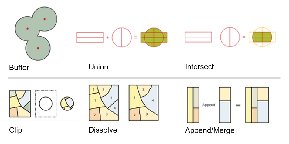
Fig. 137 Different spatial geoprocessing tools. Source: Adapted from Saylor Academy

In this chapter, we will first explore spatial joins. Spatial joins, for example, allow us to import attributes from one layer to another on the basis of their location in relation to geofeatures in another layer. These Spatial relationships can also be used to select features of a layer. Furthermore, we will go over the spatial processing tools buffer, clip, and dissolve. These operations allow us to combine geometries from two layers in various ways (see Fig. 137).

Spatial joins

Joins are ways to combine two different data layers. In general, there are two types of joins: non-spatial joins and spatial joins. Non-spatial joins rely on specific attribute values, which are used as ID-fields, to combine two layers. These are covered in the chapter “Non-spatial processing tools” in this module. Sometimes we want to combine information from different layers that don’t share a common value. In these cases, we can use spatial joins, which let us join data based on location rules. Spatial joins in QGIS enhance the attributes of the input layer by adding additional information from the join layer, relying on their spatial relationship. This process enriches your data by incorporating relevant details from one layer into another based on their geographical associations. In QGIS, a spatial join creates a new layer by comparing the features of one layer to another, depending on their spatial relationship.

For example:

• Any point within a polygon should inherit attributes of the polygon

• Only keep regions which contain an airport.

Humanitarian Example:

We have a flood depth model and we want to find out which buildings are flooded under this scenario. We can find this out by performing a spatial join to add the flood depth to the polygon layer with the houses

The resulting map could look something like this

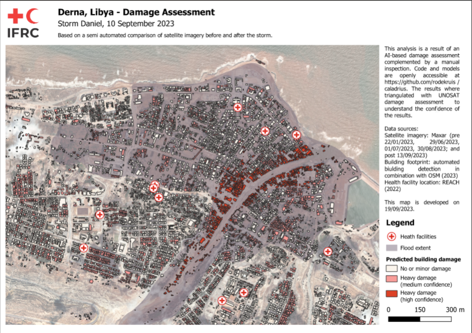
Fig. 138 A building footprint layer combined with a flood extent layer. By joining them, we can assess which houses are at risk to be damaged by flooding (Source: REACH).

Spatial joins rely on the geometrical operators. In the tabs below, you can find the different geometrical operators available in QGIS and how they affect the data processing.

Intersect

Tests whether the geometry of the two layers intersects with one another. The algorithm returns the value “True” (1), if the geometries intersect spatially. This means that they share any portion of space, overlap, or touch. If they don’t overlap, the algorithms returns the value “False” (0). In the picture below, the algorithm will return the circles 1, 2, and 3.

Disjoint

Disjoint features do not share any portion of space. This means that they don’t touch or overlap. In the picture below, the algorithm would output a layer with only the circle 4.

Equal

The algorithms returns a layer with geometries that are exactly the same (all the points and lines are equal). In the picture below, no circles are returned (added to the output layer).

Touch

Tests whether a geometry touches another. The algorithm outputs a new layer with the geometries that have at least one point in common, but their interiors do not intersect. In the image below, only circle 3 is returned.

Overlap

Tests whether geometries overlap. Returns geometries if they share space, are of the same dimension, but are not completely contained by each other. In the image below, only circle 2 is returned.

Are within

Tests whether one geometry is within another. Returns geometries a if they are completely inside of geometry b. Only circle 1 is returned.

Contain

Returns geometries if and only if no points of b lie in the exterior of a, and at least one point of the interior of b lies in the interior of a. In the picture, no circle is returned, but the rectangle would be if you would look for it the other way around, as it contains circle 1 completely. This is the opposite of “are within”.

Cross

Returns geometries that have some, but not all, interior points in common and the actual crossing is of a lower dimension than the highest supplied geometry. For example, a line crossing a polygon will cross as aline (true). Two lines crossing will cross as a point (true). Two polygons cross as a polygon (false). In the picture below, no circles will be returned.

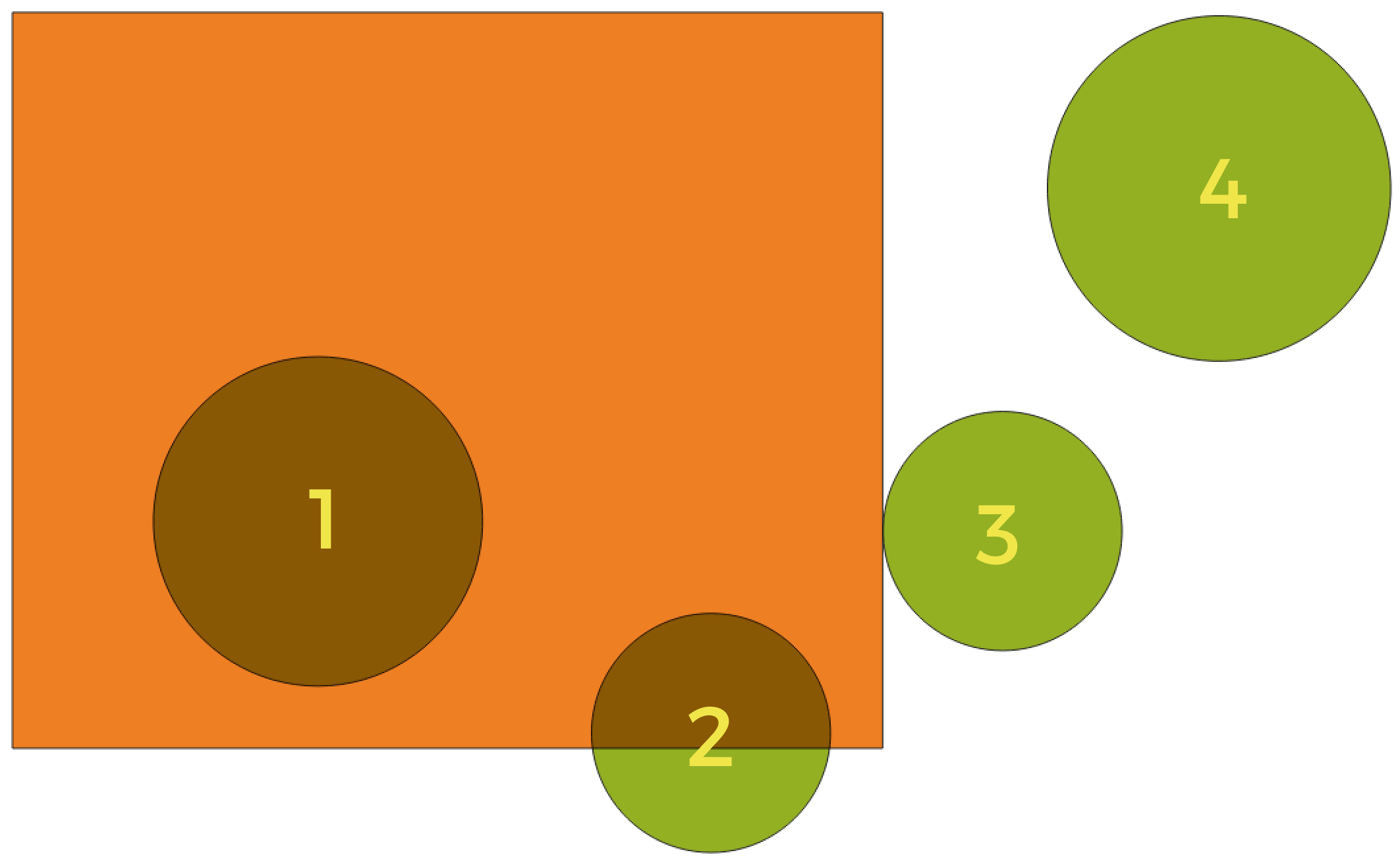
Fig. 139 Looking for spatial relations between layers
(Source: QGIS Documentation, Version 3.28)

Performing a spatial join

Now it’s your turn!

Practical exercise is crucial to understand how GIS, and QGIS, works. You can follow along by download the necessary data.

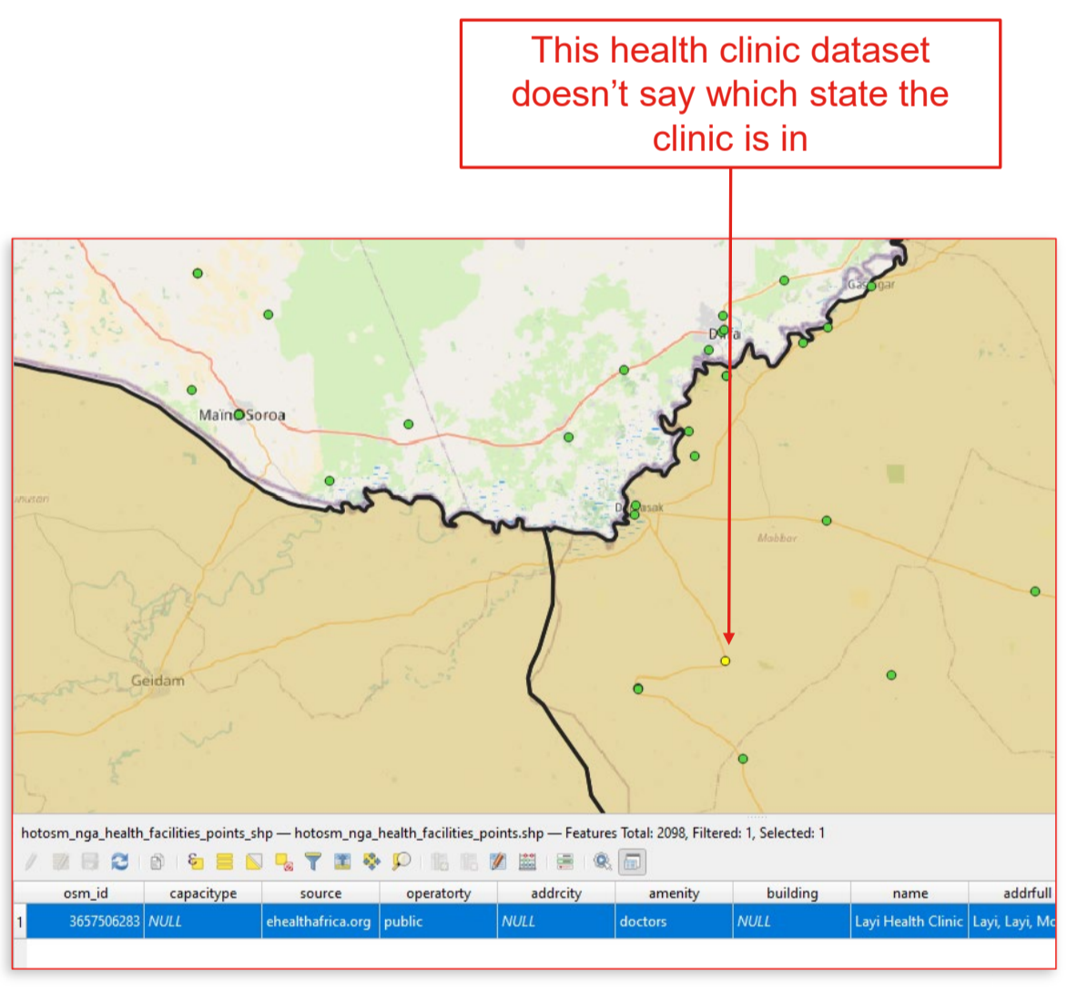
Fig. 140 An example of a situation where you will use a spatial join (Source: BRC)

In the example above (Fig. 140), we have a dataset containing the healthsites by healthsite.io and a dataset with the administrative boundaries (adm2) of Nigeria. We want to know in which state each healthsite is located. To do this, we need to use the tool “Join Attributes by Location”:

Tip

You can find activate the processing toolbox panel by navigating to View > Panels > Processing Toolbox. It should appear on the right side of your screen

1. Download the necessary datasets from HDX

   • nigeria-healthsites-shp

   • nga_adm_osgof_20190417.zip

2. Unzip the files, create a new QGIS-project, and load the files into the QGIS-project.

3. Search for the tool “Join Attributes by Location” in the processing toolbox and Double-Click on it. A new window will open (see Fig. 141).

4. Use the health facilities layer as the target (“Join to feature in”) and the adm2 layer as the comparison layer (“By comparing to”).

5. Use the are within geometrical predicate.

6. Select the fields to add: ADM2_EN, ADM2_PCODE

7. Select Discard records that could not be joined

8. Click Run to proceed; the log should confirm success.

9. A new (temporary) layer called “Joined features” will appear in your layers-panel

10. Right-click on the layer and select “Export” or “Make Permanent” to save the new layer.

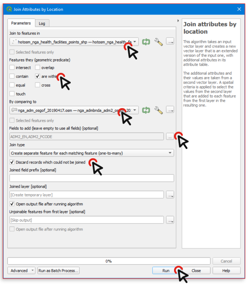
Fig. 141 Setting the parameters to perform the spatial join in QGIS 3.36

Congratulations, we now have added the information about the administrative region to the health facilities layer! We can symbolise the joined layer with the categorised symbology to verify if it worked (see Fig. 142). Note that the points in the original dataset which were outside of Nigeria’s border have been discarded as they could not be joined.

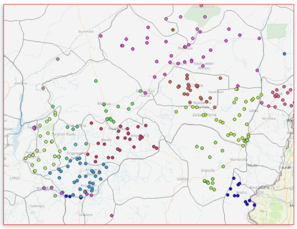
Fig. 142 The different colours for the points indicate that they are located in a different state (adm2).

More spatial join-tools in QGIS

By default, QGIS provides three different tools to perform spatial joins. The first, and the most common one, is the tool “Join attributes by location”. Furthermore, there are also the tools “Join attributes by location (summary)” and “Join attributes by nearest”.

Join attributes by location

This tool takes two input layers and creates a new vector layer which has the attributes of both layers in its attribute table. The first input layer (see “Join to features in” in Fig. 143) dictates which geometric features will be copied to the new layer. The second input layer (see “By comparing to” in Fig. 143) dictates the attributes that will be added to the new layer on top of the attributes of the first input layer. You can select which of these attributes should be transferred to the new layer.

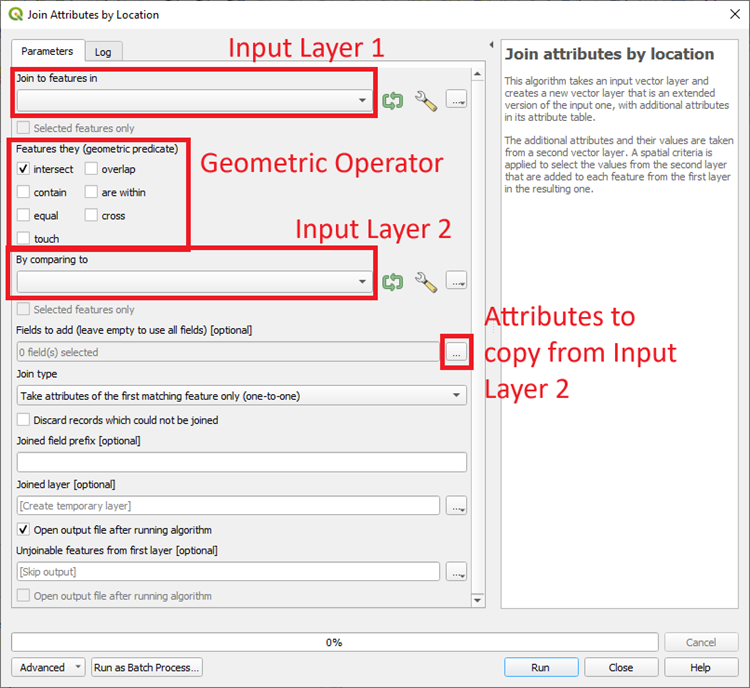
Fig. 143 The “Join Attributes by Location”-tool in QGIS 3.36.

Join attributes by location (summary)

This tool is similar to the “Join Attributes by Location”-tool. However, on top of adding the attributes from one layer to another, this algorithms also calculates statistical summaries for the values from matching features in the second layer. These summaries include a wide range of options, such as minimum and maximum values, mean values, as well as counts, sums, standard deviation, and more.

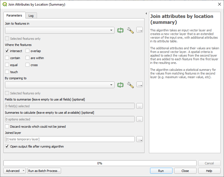
Fig. 144 Screenshot of the tool Join attributes by location (summary) in QGIS 3.36

Join attributes by nearest

This type of spatial join is similar to the other two joins but the joining of features occurs by identifying the closest features from each of these layers. Furthermore, if a maximum distance is specified, only the features that are within this designated distance will be considered as suitable matches for the joining process.

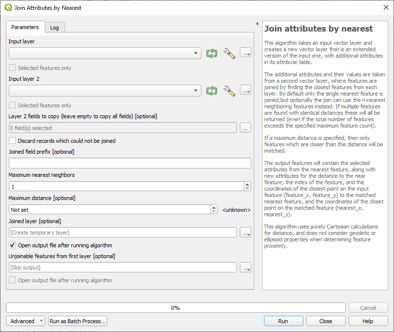
Fig. 145 Screenshot of the tool Join attributes by nearest in QGIS 3.36

Note

A detailed description of the functions and settings of these tools can be found in the QGIS documentation

Exercise: Calculate sum of affected population and flooded area for the Area of interest

In the aftermath of flooding events, data on the affected population and the extent of flooding is crucial. This information can be refined from a nationwide dataset to provide specific numbers for individual districts or states. This can aid in identifying the areas most heavily impacted, leading to more efficient relief operations. In the upcoming exercise, we will calculate the total flooding extent in square kilometers and the affected population for Unity State, South Sudan. To accomplish this, we will utilize the Join attributes by location (summary) tool.

1. Load the necessary data for this exercise into your QGIS. Both datasets were downloaded from HDX:

   • South Sudan - Subnational Administrative Boundaries:
     State_Unity_South_Sudan.shp

   • Satellite detected water extents between 11 and 15 August 2023 over South Sudan: Download the folder FL20220424SSD_SHP.zip, unzip it, and search for the file VIIRS_20230811_20230815_MaximumFloodWaterExtent_SouthSudan.shp

2. Locate the tool named Join attribute by location (summary)

   • Choose state boundaries as the target layer for joining features

   • Set intersect as the spatial relationship

   • Select flood extent layer as the comparison layer

   • Specify the fields to be summarized as Area_km2 and Pop

   • Choose sum as the type of summaries to be calculated

   • Click Run to start the process

3. Once completed, you will have access to information on the total affected population and flooded areas for the entire state of Unity.

Solution: Calculate sum of affected population and flooded area for the Area of interest

Overlay Operations (Clip, Dissolve, Buffer)

Overlay operations allow us to combine geometries of two layers in different ways (see Fig. 146). The difference to spatial joins is that the geometries are transformed in the process.

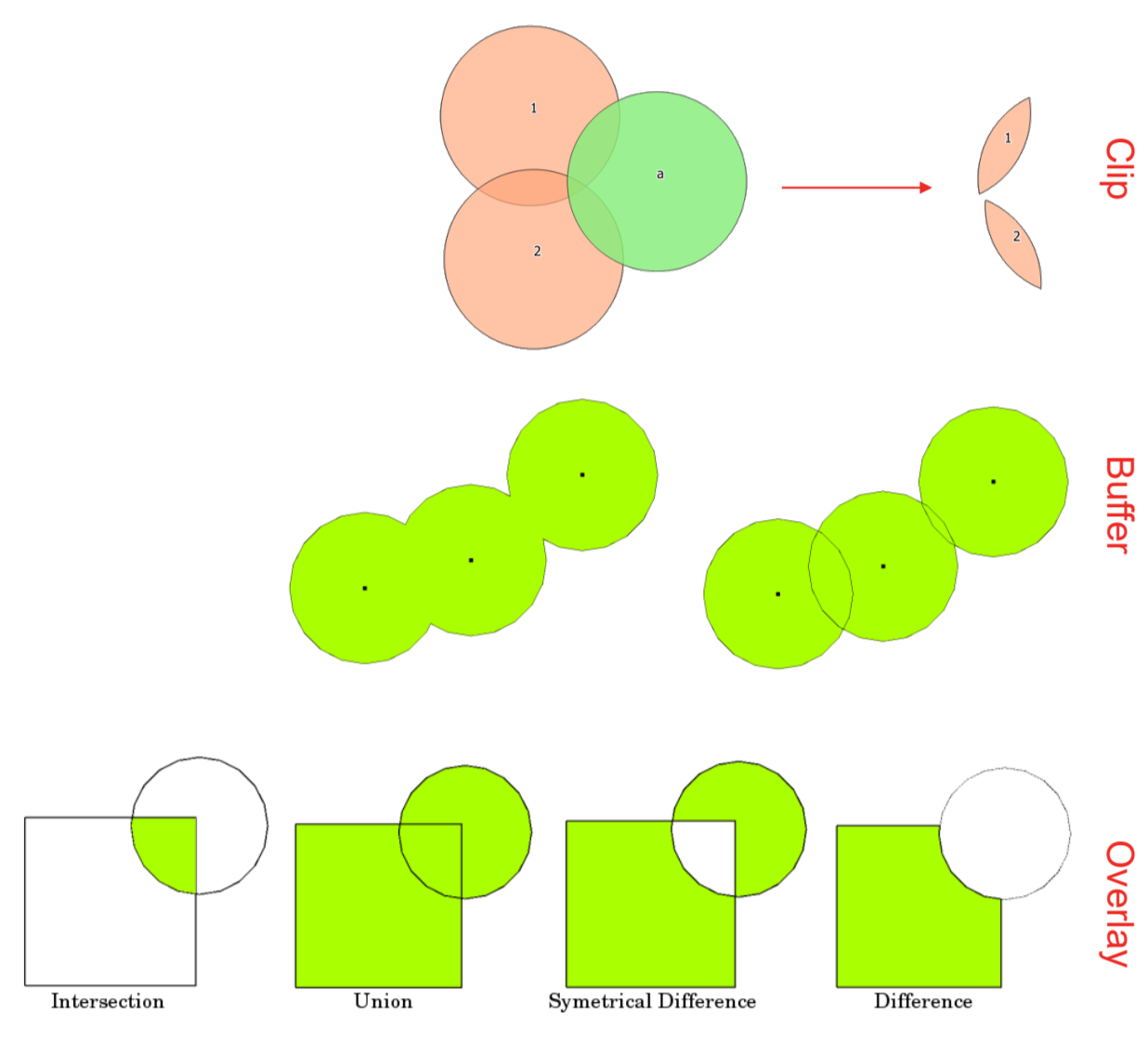
Fig. 146 Visual representation of different overlay operations.

Overlay operations include Clipping, Buffering, and Dissolving. In the next subchapters, we will take a look at each of these overlay operations in turn and provide some examples for humanitarian work.

Clip

The Clip tool is used to cut a vector layer using the boundaries of another polygon layer. In other words, it extracts a portion of a dataset based on the boundaries of another. It keeps only the parts of the features in the input layer that are inside the polygons of the overlay layer, producing a refined dataset. While the core attributes of the features remain the same, some properties, like area or length, may change after the clipping operation. If you’ve stored these properties as attributes, you might need to update them manually.

Humanitarian Example:

We have flood extent data for Pakistan, but we are currently working on a map showing the flood damage in a specific administrative region. In this case, we can take the flood layer and clip it to the administrative boundaries of the area of interest.

The tool has two different input options:

• Input layer: Layer from which the selection is clipped

• Overlay layer: Area of interest to which the input layer will be clipped

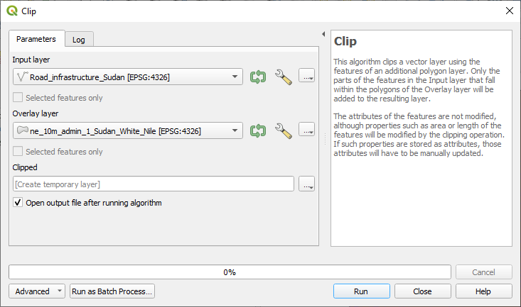
Fig. 147 Screenshot of the Clip tool with the input data.

Exercise: Clipping a roads layer to administrative boundaries

Information on road infrastructure for humanitarian aid operations is of great importance and can be easily retrieved from open-source data sources like OpenStreetMap. However, this information is often included in extensive datasets that contain a significant amount of irrelevant details for specific operations or it covers a lot more area than is necessary for the operation. To make working with this data more efficient, it is common practice to clip the data to the area of interest. In addition to clipping, data can often be filtered, in order to remove data we are not interested in.

1. Load the OSM roads data from the HOT Export tool (part of the Humanitarian OpenStreetMap Team) here as a new layer: Road_infrastructure_Sudan.geojson.

2. Filter the layer by using the query builder to only show primary and residential roads (“highway” = ‘primary’ OR “highway” = ‘residential’)

3. Load the admin1 layer for Sudan which contains the district White Nile, ne_10m_admin_1_Sudan_White_Nile.geojson. They are downloaded from Natural Earth Data.

4. Select the roads layer and open the Clip dialogue from Vector > Geoprocessing Tools

   • Set roads as the input layer and the district boundaries of White Nile as the overlay layer

   • Click Run to generate a temporary layer called Clipped

5. You now have a tidy roads layer which contains the necessary information

Solution: Clipping a roads layer to administrative boundaries

In addition to the standard QGIS operation Clip, there are two other more advanced tools for performing clipping processes. These tools are GDAL operations, which enable the definition of the clipping extent. This extent can be either a specific area or a mask layer. The second option is quite similar to the standard clipping process provided by QGIS.

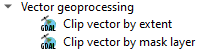
Fig. 148 The GDAL tools Clip vector by extent and Clip vector by mask layer

Clip vector by extent

This operation clips any vector file to a given extent. This clip extent will be defined by a bounding box that should be used for the vector output file. It also has to be defined in the target CRS coordinates. There are different methods to define the bounding box, which are the great difference between this tool and the standard clipping process:

• Calculate from a layer: this uses the extent of a layer loaded into the current project

• Calculate from layout map: uses the extent of a layout map item in the active project

• Calculate from bookmark: uses the extent of a saved bookmark

• Use map canvas extent

• Draw on canvas: click and drag a rectangle delimiting the area to take into account

• Enter the coordinates as xmin, xmax, ymin, ymax

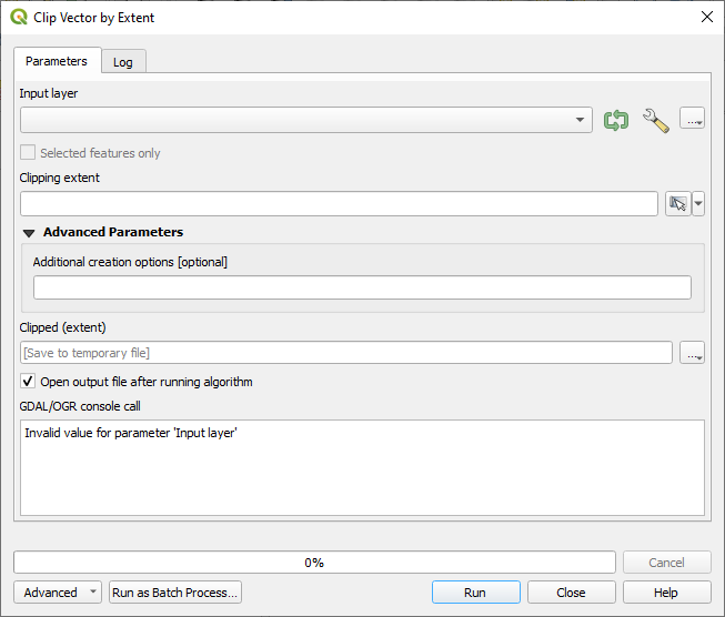
Fig. 149 Screenshot of the tool Clip vector by extent

Clip vector by mask layer

This operation uses a mask polygon layer to clip any vector layer. This operation only takes two input:

1. The input layer

2. The mask layer which is used as the clipping extent for the input vector layer

Fig. 150 Screenshot of the tool Clip vector by mask layer

Dissolve

The Dissolve-tool creates a new layer and merges overlapping features from one or two vector layers. You can pick one or more attributes to group together features that share the same value for those attributes. Alternatively, you can combine all features into one. If you’re working with polygons, it will remove shared boundaries between them.

If you turn on the “Keep disjoint features separate” option when running the tool, it’ll make sure that features or parts that don’t overlap or touch each other are saved as separate features instead of being part of one big feature. This allows you to create several vector layers.

Humanitarian Example:

Our data shows roads in segments by type. We dissolve the segments to create a single road layer, categorized by road type.

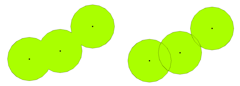
Fig. 151 Buffer zones with dissolved (left) and with intact boundaries (right) showing overlapping areas
(Source: QGIS Documentation, Version 3.28)

In the next section on buffers we will be using the dissolve-tool.

Buffer

Buffering creates zones of predetermined distances around geometric features as a new polygon layer. These buffers surround the input vector features. This buffer zone is typically uniform and extends outward from the original input features, making it useful for various spatial analyses and mapping applications. Buffers can be created around points, lines, and polygons as shown in Fig. 152.

Examples for analyses using buffers could be:

• Creating of buffer zones to protect the environment

• Analysing greenbelts around residential area

• Creating risk areas for natural disasters.

Humanitarian Example:

We need to assess which areas live close enough to clean water sources so the population can easily reach them by walking. In this case, we can create buffer zones of 2 km around a dataset with wells to see which areas are covered

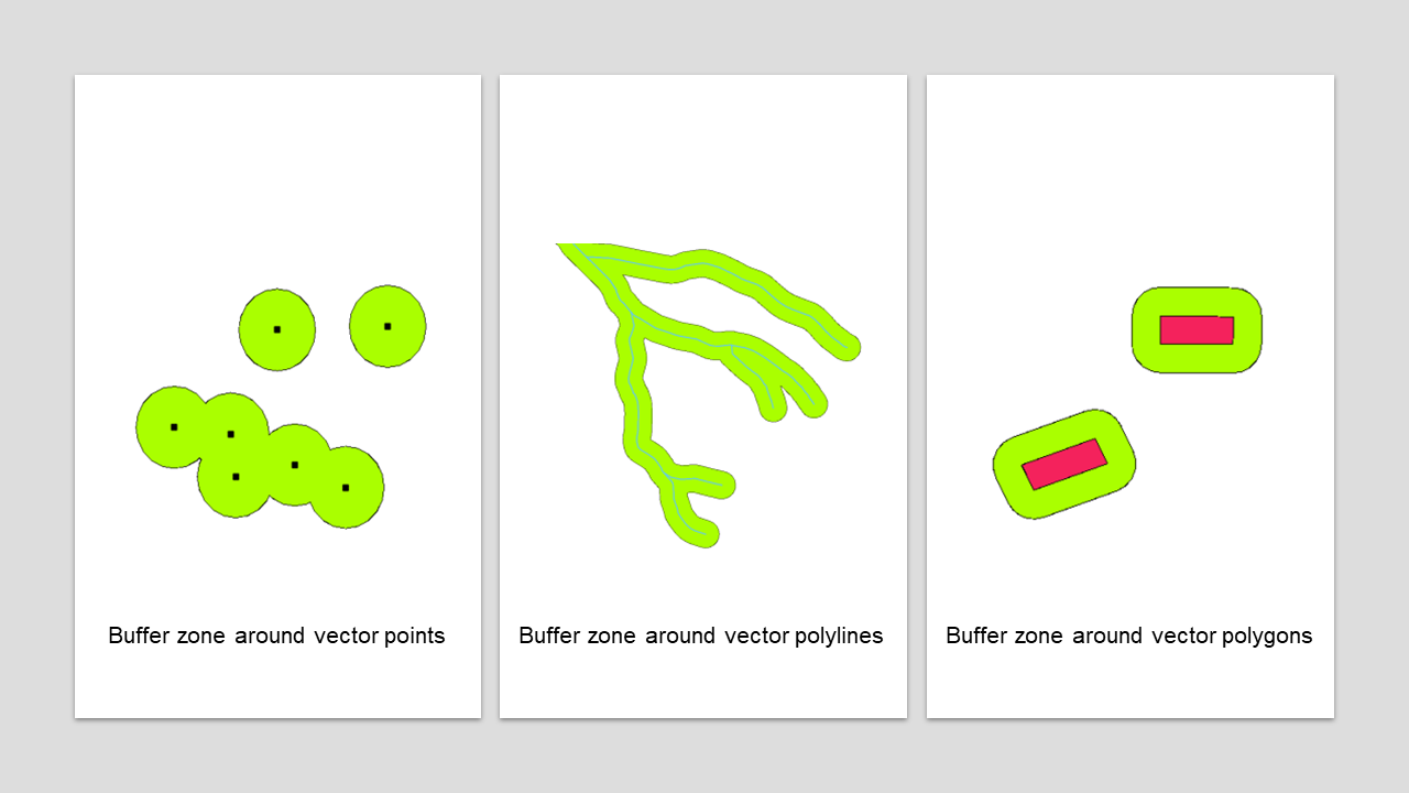
Fig. 152 Different kinds of buffer zones
(Adapted after QGIS Documentation, Version 3.28)

There are several variations in buffering. The buffer distance or buffer size can vary according to the numerical values provided. The numerical values have to be defined in map units according to the Coordinate Reference System (CRS) used with the data.

Attention

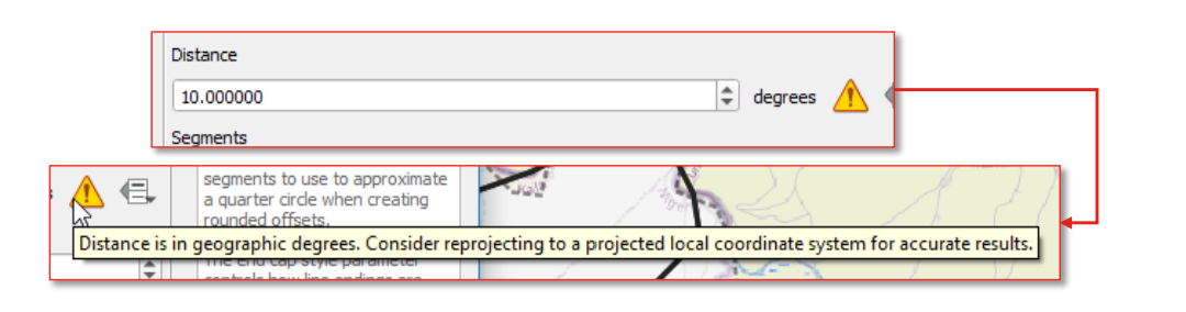
Fig. 153 The error message QGIS displays when performing distance based calculations in a geographic coordinate system

If…

• You get a projection warning message

• Your layer(s) don’t show up

• Layers look odd ‒ e.g. squashed

• Error message “using degrees” when using distances (as shown in Fig. 153) … it might be a projection issue.

To solve it, try…

• Changing the CRS for the layer

• Reprojecting the layer

For example, if you are trying to make a buffer on a layer with a Geographical Coordinate System, QGIS will warn you and suggest to reproject the layer to a metric Coordinate System. This is because when you are using a metric coordinate system, the algorithm will use degrees to calculate the distance of the buffer size. However, the distance between degrees are not uniform and depend on the latitude (see Fig. 154)

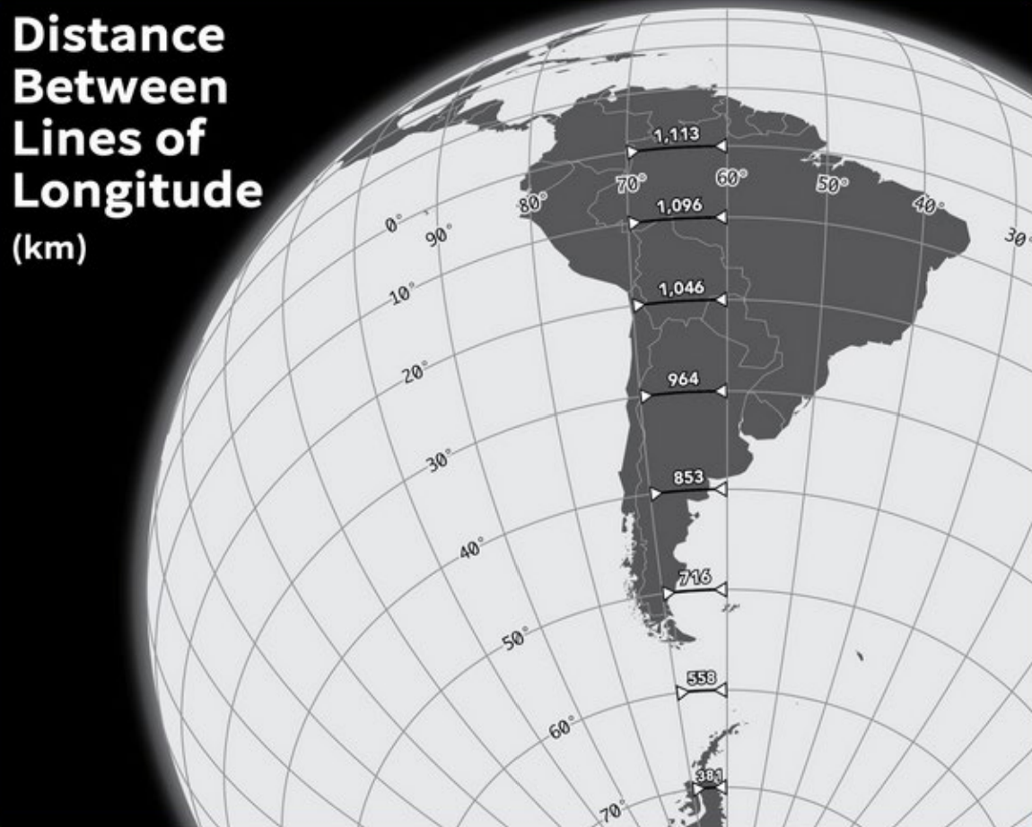
Fig. 154 This image illustrates this – 10 degrees of longitude at the equator is 1,113km, but 10 degrees of longitude at 70 degrees latitude is only 381km. (Source: Ricky Angueria).

This is why you’ll need to convert to a local/projected coordinate system to be able to specify distances in km/miles (e.g. when using the buffer tool).

Exercise: Create 10km buffer around health centres

Another example relevant for humanitarian action can be the creation of a map which provides information about the coverage of health sites in the distance of 10 km. To achieve this, a buffer of 10 km is created around points representing healthsites. In some cases, this will create buffer zones which overlap. In order to create a homogenous area, we can dissolve overlapping buffer zones.

1. Download the Sudan health sites data from HDX as a shapefile

2. Load your new data into QGIS. Also add the district boundaries of Khartoum, ne_10m_admin_1_Sudan_Khartoum.geojson. They are also downloaded and adapted from Natural Earth Data.

3. Clip your health sites to the boundaries of Karthoum district

4. Reproject the health sites layer to a local coordinate system to enable setting distances in km

   • Vector menu > Data Management Tools > Reproject Layer

   • Select the health sites layer as the input layer

   • Set the target CRS to WGS 84 / UTM zone 36N (click the projections icon to search the full list of options)

   • Click Run to reproject

5. Open the Buffer tool by accessing Vector > Geoprocessing Tools > Buffer

   • Select the reprojected layer as the input layer

   • Set the distance to 10km

   • Check the option to dissolve result

   • Leave the other options as defaults and click Run

6. Now you have a rough overview over the coverage with health sites for the district of Khartoum

Solution: Create 10km buffer around health centres

Centroids

This process creates a new point layer, with points representing the centroids of the geometries of the input layer.

The centroid is a single point that shows the middle of all the parts of a feature. It can be outside the feature or on each part of it.

The attributes of the points in the output layer are the same as for the original features.

Centroids are especially useful when creating graduated symbols maps, as the size of the point symbols can be graded using the graduated classification method.

Fig. 155 The black points represent the centroids of the features from the input layer.