Exercise: Nigeria Floods

🔙Back to Homepage

Aim of the exercise:

In this exercise, you will learn how to digitise the positions of settlements by creating new datasets. Furthermore, you will learn how to enrich the simple geodata set with additional information.

Relevant Wiki Articles

• QGIS Interface

• Types of Geodata

• Geodata Import in QGIS

• Layer Concept

• Non-Spatial Querie

• Spatial Queries

• Table function - Add field

• Geodata Classification- Categorized

• Geodata Classification- Graduated

• Digitization- Point data

• Geoprocessing - Clip

Data sources

Download the data folder here and save it on your PC. Unzip the .zip file! The folder is called “Modul_3_Exercise_1_Flood_Nigeria” and contains the whole standard folder structure with all data in the input folder and the additional documentation in the documentation folder.

• Nigeria: Administrative Division with Aggregated Population (“kontur_boundaries_NG_20230628.gpkg”)-Kontor

• Nigeria : Flood data (“Nigeria_flood_2022_affacted_population”) - UN OCHA. This dataset was manipulated for training purposes.

• Satellite detected water extents between 1 and 25 October 2022 over Nigeria (VIIRS_20220901_20220930_MaximumFloodWaterExtent_Nigeria.shp) UNOSAT

Task

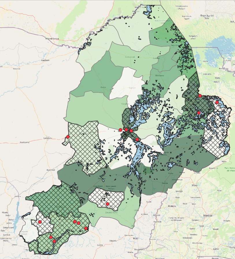
Our goal is to produce an overview of the impact of the 2022 flood in the state of Burco in Nigeria. To this end, we will visualize the state and the affected districts, plus we will digitize communities which are reportedly affected.

1. Open QGIS and create a new project by clicking on Project -> New

2. Once the project is created save the project in the “project” folder of the exercise “Modul3_Exercise_1_Flood_Nigeria”. To do that click on Project -> Save as and navigate to the folder. Name the project “Nigeria_Borno_flood_2022”.

3. Load the GeoPackage “kontur_boundaries_NG_20230628.gpkg” in your project by drag and drop (Wiki Video). Or click on Layer-> Add Layer-> Add Vector Layer. Click on the three points and navigate to “kontur_boundaries_NG_20230628.gpkg”. Select the file and click Open. Back in QGIS click Add (Wiki Video). This dataset contains all administrative division areas (admin 0 to 5) with the respective population of the areas.

Attention

GeoPackage file can contain multiple files and even whole QGIS projects. When you load such a file in QGIS a window will appear in which you have to select the files you want to load in your QGIS project.

4. First, we want to export Borno state from kontur_boundaries_NG_20230628 to have it as a stand-alone vector layer. To do that,

   • Open the attribute table of “kontur_boundaries_NG_20230628” by right click on the layer -> Open Attribute Table(Wiki Video).

   • Find the row of Borno state and mark it by clicking on the number on the very left-hand side of the attribute table. The row will appear blue and the area of Borno state will turn yellow on the map canvas. You can right-click on the row and click Zoom to Feature(Wiki Video). .

   • Now right-click on the layer in the Layer Panel and click on Export -> Save Selected Features as. We want to save Borno as a GeoPackage, so adjust Format accordingly. Click on the three points and navigate to your temp folder. Here you can give it the layer the name “AOI_Borno_admin1” and click Save. Now you should see the same name in the Layer name field. Click ok(Wiki Video) .

5. In the next steps, we want to create a vector layer with admin 2 areas or in Nigeria called Local Government Areas (LGA) with the population in our project. Since we only want the LGAs we need to export those from the original dataset.

   • Open the attribute table of the layer “kontur_boundaries_NG_20230628” by by right click on the layer -> Attribute Table (Wiki Video). Check out the attribute table. You see two columns of admin levels “admin levels” and “osm_admin_levels”. Both have different values. In the metadata of the dataset on HDX we can find out that the column “osm_admin_levels” refers to the admin levels used in OpenStreetMaps (OSM). There is a list of which official admin levels correspond to which OSM admin levels. The LGAs correspond to osm admin level 6. This means we want to export all features with osm_admin_level = 6.

   • To export exactly these features we will use the tool Extract by attribute. Open the Processing Toolbox (here is how) and search for the tool. Open the tool and choose as Input Layer the “kontur_boundaries_NG_20230628.gpkg“ layer. Under Selection attribute choose the column osm_admin_level. The Operator has to = and as value we set 6 since the LGAs have the osm_admin_level 6.

   • Under Extracted (attribute) click on the three points-> Save to GeoPackage navigate to your temp folder, and call the new layer “Nigeria_admin2_pop”. Click Save. Give the layer the same name ( “Nigeria_admin2_pop”). Click OK and then click Run.

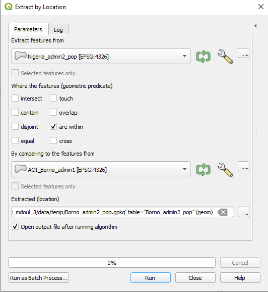
6. Now we need to extract all LGAs in Borno. For that, we will use the Tool Extract by Location (Wiki Video) . Search the tool in the Processing Toolbox and open it.

   • As Input Layer we will use “Nigeria_admin2_pop”.

   • For By comparing to the features from we use the layer “AOI_Borno_admin1”.

   • As Geometric predicate we use are within.

   • To save the output click on the three points at Extract (location) -> Save to GeoPackageand navigate to your temp folder. Save the new layer under the name “Borno_admin2_pop”. Give the new layer the same Layer name and click Run.

   • Open the Attribute table of the new layer. You should have 27 features.

7. We have our admin areas in place and can now start to enrich these layer with additional data regarding the flood of 2022. Open the Excel or pdf file “Nigeria_flood_2022_affacted_population” and open the sheet Borno. You find a table with the LGAs and communities which were affected by the flood. Now we want to add some of the information to our “Borno_admin2_pop” layer. For that, there are two ways. One simple but more time-consuming and one more complicated but much faster way. We will show here the easy way but in the dropdown below you find the tutorial for the advanced way as well.

   • Open the attribute table of “Borno_admin2_pop” and activate the editing mode by clicking on (Wiki Video). Now you are able to edit the data directly in the table.

   • First, we add a new column with the name “Flood_affacted”. To do so click on . In the Add field window you have to add the name and set the Type to Text(string). Click OK (Wiki Video) .

   • In the next step check in the Excel/PDF table which LGAs were affected and put “Yes” in the attribute table for those LGAs.

   • When you are down click to save your edits and switch off the editing mode by again clicking on (Wiki Video).

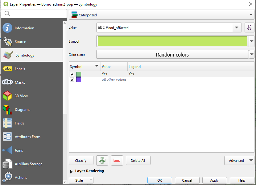
8. To visualize the enriched data set, we use the function “Categorized Classification” function. This means that we select a column from the attribute table and use the content as categories to sort and display the data (Wiki Video).

   • Right-click on the layer “Borno_admin2_pop” in the Layer Panel -> Properties. A new window will open up with a vertical tab section on the left. Navigate to the Symbology tab.

   • On the top you find a dropdown menue. Open it and choose Categorized. Under Value select “Flood_affacted”.

   • Further down the window click on Classify. Now you should see all unique values or attributes of the selected “Flood_affacted” column. You can adjust the colours by double-clicking on one row in the central field. Once you are done, click Apply and OK to close the symbology window.

9. Next, we want to visualize the affected communities which are listed in the Nigeria_flood_2022_affacted_population table. To find these communities in QGIS we need two things. An OpenStreetMap base map and the plugin OSM Place Search.

   • To add the OSM as a base map click on Layer -> Add Layer -> Add XYZ Layer…. Choose OpenStreetMap and click Add. Arrange your layer in the Layer Panel so the OSM is at the bottom (Wiki Video) .

   Tip

   You can not interact with a base map!

   • To add the plugin OSM Place Search, click on Plugins -> Manage and Install Plugins… -> All and search for OSM Place Search. Once you have found it click on it and click Install Plugin. You can open the OSM Place Search Panel like every other panel by clicking on View -> Panels and checking OSM Place Search Panel(Wiki Video).

   • In the panel, you can search for places on the OpenStreetMap by typing the name of the place in the search bar. Often it makes sense to add additional information like the name of the country. Try for example “Laujeri Bulama, Nigeria”.

10. Now we have all our tools in place. In the next step, we create a new point vector layer from scratch to digitize the location of the affected communities.

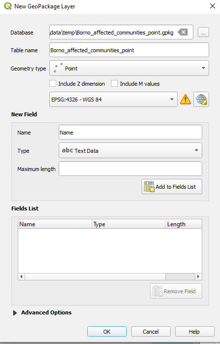
    • Click on Layer –> Create Layer -> New GeoPackage Layer(Wiki Video)

    • Under Database click on and navigate to temp folder. Give the new dataset the name “Borno_affected_communities_point”. Click Save.

    • Geometry type: Select Point

    • Under Additional dimension you should always make sure that you check None.

    • Select the coordinate reference system (CRS) “EPSG:4326-WGS 84”. By default, the QGIS selects the project CRS.

    • Under New Field you can add columns to the new layer. Add the column “Name”.

      • Name = “Name”

      • Type: Select Text Data

      • Click on Add to Fields List to add the new column to the Fields List.

      • Click OK.

    • Your new layer will appear in the Layer Panel

11. Currently the new “Borno_affected_communities_point” is empty. To add features we can use the Digitizing Toolbar. . If you can not see the toolbar View -> Toolbars and check Digitizing Toolbar` (Wiki Video).

    • Select the point layer “Borno_affected_communities_point” in the Layer panel. Go to the digitalisation toolbar and click on. No the layer is in the editing mode .

    • Search an affected community based on the table “Nigeria_flood_2022_affacted_population”. Once you have found one, click on . Left-click on the feature you want to digitalise.

    • Once you click, a window will appear Borno_affected_communities_point Feature Attribute. Here you can add the name of the location.

    • Repeat the same process for as many communities as you like.

    • Once you are done with digitizing click on to save your edits.

    • Click again on to end the editing mode.

12. In this step, we want to add information about the population to the map. This will help us to visualize where the most people are potentially affected. Since the layer “Borno_admin2_pop” contains this information we can dublicate this layer.

    • To do that right click on the layer -> Duplicate Layer. The name of the new layer will be “Borno_admin2_pop_copy”.

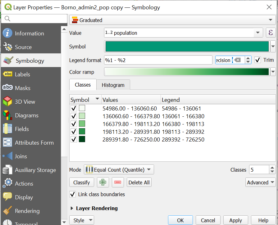
13. Since absolute population numbers are natural numbers, we can not use categorised classification. Instead, we use the option Graduated (Wiki Video).

    • Right-click on the layer “Borno_admin2_pop_copy” in the Layer Panel -> Properties. A new window will open up with a vertical tab section on the left. Navigate to the Symbology tab.

    • On the top you find a dropdown menue. Open it and choose Graduated.

    • Under Value select “Population”.

    • Color ramp: Select a white-to-green color ramp. Since we want to visualize the population, it is important to use neutral colours.

    • Mode: Equal Count (Quantile)

    • Classes: 5

    • Click Classify

    • Click Apply

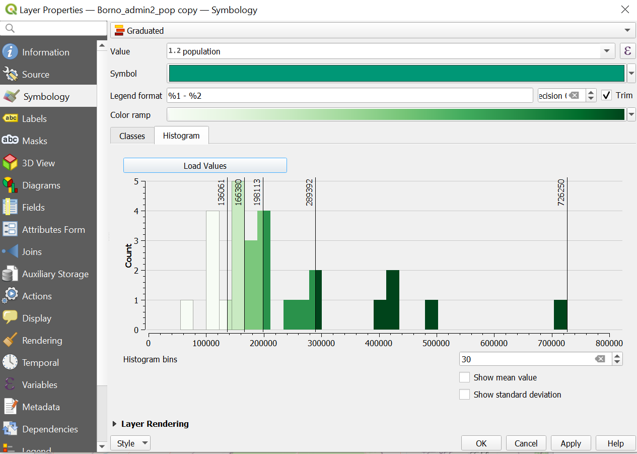
14. QGIS created now five classes covering the whole range of population numbers in Borno state. Click on the Histogram Tab -> Load Values. Here you see the distribution of values in the dataset and the limits of the classes. We see that most LGAs have a population below 300.000 people. Try out some of the other modes of classification like natural breaks or equal intervals.

15. To visualise “Borno_admin2_pop” sowing affected LGAs and “Borno_admin2_pop_copy” sowing population data together, we need to change the symbology of “Borno_admin2_pop”. First, right-click on the layer “Borno_admin2_pop” in the Layer Panel -> Properties. A new window will open up with a vertical tab section on the left. Navigate to the Symbology tab. Currently, we use the Categorized classification. We want to keep that. However, we only want to show affected LGAs. Hence, we uncheck the row that corresponds to the LGAs without Affected = Yes.

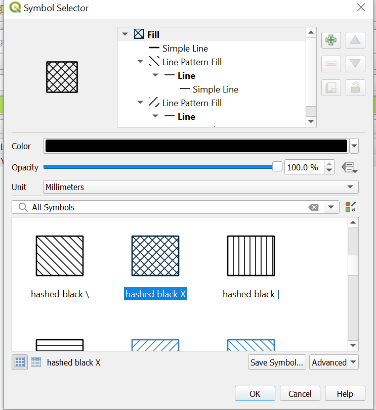
    • Right-click on the layer “Borno_admin2_pop” in the Layer Panel -> Properties. A new window will open up with a vertical tab section on the left. Navigate to the Symbology tab.

    • Then, do a double-click on the Yes row. Here we have two options. We can use a grid or only the borders.

    • To use a grid scroll down and select one that suits you. Then click OK.

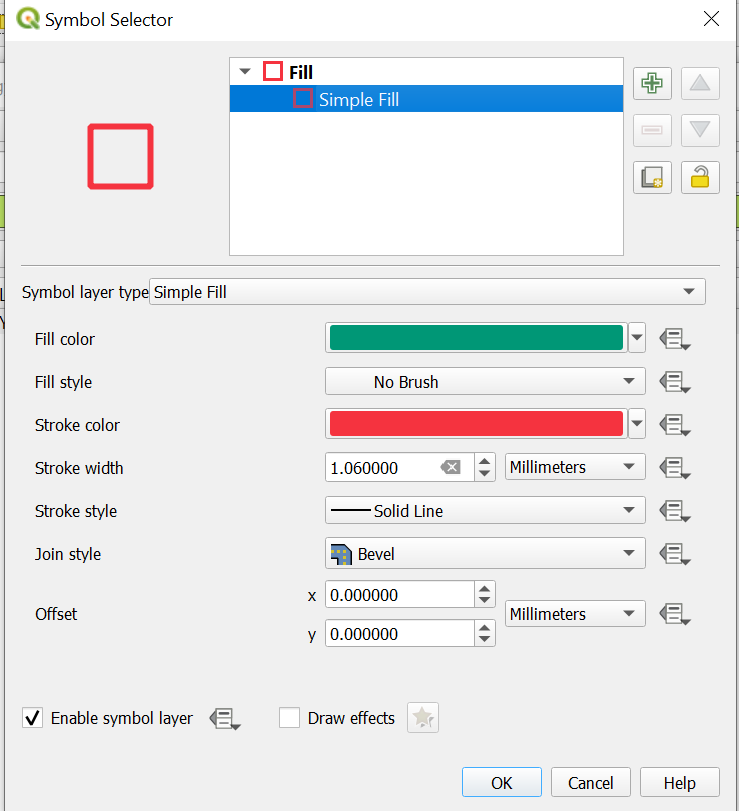
• To only use borders, click on simple fill -> Fill style and select No Brusch. Adjust the Stroke Color to a red or another bride colour. Increase the Stroke width to make the borders bigger. Then click OK.

16. For a more detailed idea of the flood extend we can load the layer “VIIRS_20220901_20220930_MaximumFloodWaterExtent_Nigeria.shp” which shows the maximum extent of surface water between 9th and 30th October 2022. If you like you can also load “VIIRS_20220901_20220930_PermanentWater_Nigeria.shp”. This layer shows lakes and other permanent surface water features. Once you loaded the layers in QGIS, you can see that they are correctly displayed. However, upon checking the layer information you can see that the new layers have a different Coordinate Reference System (CRS). They have the EPSG Code 9707 whereas our project has 4326 (Wiki Video).

    • Right click on the data layer, click on “Properties”.

    • The “Layer Properties” Window of the data layer will open. Click on “Information”.

    • Under the headline “Coordinate Reference System (CRS)” you find all information about the CRS. The most important are:

    • Name: Here you find the EPSG Code

    • Unites: Here you can find wether it is possible to use meters with this data layer or latitude and longitude.

17. This will be a problem as soon as we do something different then just displaying the layers. Since we want to manipulate the layers in the next step we need to reproject them first (Wiki Video).

    • Click on the Vector Tab -> Data Management Tools -> Reproject Layer or search for the tool in the Processing Toolbox .

    • As Input layer select “VIIRS_20220901_20220930_MaximumFloodWaterExtent_Nigeria.shp”

    • Select as target CRS/ EPSG-Code 4326.

    • Save the new file in your temp folder by clicking on the three dots next to Reprojected, specify the file name as “Flood_extand_Nigeria_october_2022_reprojected.

    • Click Run

    • Delet the old layer from the layer panel by right click on the layer -> Remove layer.

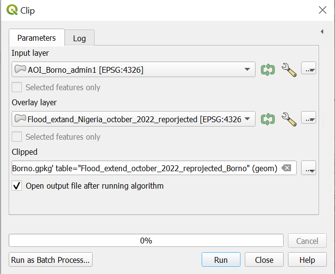
18. The flood extend layer covers the whole of Nigeria. We can use the Clip tool to cut it to the shape of Borno state (Wiki Video).

    • Open the Processing Toolbox (here is how) and search for the Clip tool.

    Note

    There are two versions of the Clip tool. Since we work with vector data, make sure to use the one under “Vector overlay”.

    • Input layer: “VIIRS_20220901_20220930_MaximumFloodWaterExtent_Nigeria.shp”

    • Overlay layer: “AOI_Borno_admin1”

    • To save the output click on the three points at Clipped-> Save to GeoPackageand navigate to your temp folder. Save the new layer under the name “Flood_extend_october_2022_reprojected_Borno”. Give the new layer the same Layer name and click Run.

Great, we have done our visualisation. WELL DONE! Your results should look similar to the image below.