Exercise 2: Automation of Exposed Population Estimation – Aina’s Model #
Characteristics of the exercise #
Type of trainings exercise:
This exercise can be used in online and presence training.
It can be done as a follow-along exercise or individually as a self-study.
Exercise Track:
This exercise is part of the Madagascar Anticipatory Action Cyclon Analysis Exercise Track
Estimated time demand for the exercise
Relevant Wiki Articles
Aim of the exercise: Aina, the GIS expert at the Malagasy Red Cross (CRM), is preparing for the upcoming cyclone season. She wants to improve her team’s ability to act quickly once a storm is forecasted by automating key analyses in QGIS. These include estimating exposed populations, identifying impacted services like health and education, and assessing whether health posts can be reached from key warehouses within a critical 10-hour window. The goal is to prepare an end-to-end analysis and visualization workflow that can support fast, data-driven anticipatory action before a cyclone makes landfall.
Instructions for the trainers #
Trainers Corner
Prepare the training
Take the time to familiarise yourself with the exercise and the provided material.
Prepare a white-board. It can be either a physical whiteboard, a flip-chart, or a digital whiteboard (e.g. Miro board) where the participants can add their findings and questions.
Before starting the exercise, make sure everybody has installed QGIS and has downloaded and unzipped the data folder.
Check out How to do trainings? for some general tips on training conduction
Conduct the training
Introduction:
Introduce the idea and aim of the exercise.
Provide the download link and make sure everybody has unzipped the folder before beginning the tasks.
Follow-along:
Show and explain each step yourself at least twice and slow enough so everybody can see what you are doing, and follow along in their own QGIS-project.
Make sure that everybody is following along and doing the steps themselves by periodically asking if anybody needs help or if everybody is still following.
Be open and patient to every question or problem that might come up. Your participants are essentially multitasking by paying attention to your instructions and orienting themselves in their own QGIS-project.
Wrap up:
Leave time for any issues or questions concerning the tasks at the end of the exercise.
Leave some time for open questions.
After manually estimating exposed populations in past cyclone seasons, Aina has decided to prepare an automated model using the QGIS Graphical Modeller. This will help her move faster and avoid repeating the same steps manually each time a cyclone is forecasted.
In this task, you will help Aina build a simple version of that model using the tools from Task 1. The model should:
Reproject the cyclone track to EPSG:29738
Buffer the cyclone track
Reproject the buffer back to EPSG:4326
Clip the population raster
Run Zonal Statistics to get exposed population per district
Tasks #
Set up the model structure:
Open the Graphical Modeler from the top menu:
Processing→Graphical Modeler…
Naming the model:
A new model window will open. On the left side, click on
Model Propertiesto define basic information about the model:Model Name:
Estimate_Exposed_PopulationGroup:
Cyclone Trigger ToolsLeave the description empty or write: “Automated model to estimate exposed population based on cyclone buffer.”
Save the model
To save the model:
Click the Save icon (💾) or go to
Model→Save.Navigate to the
modelsfolder of your training structure.Save the model as:
Estimate_Exposed_Population
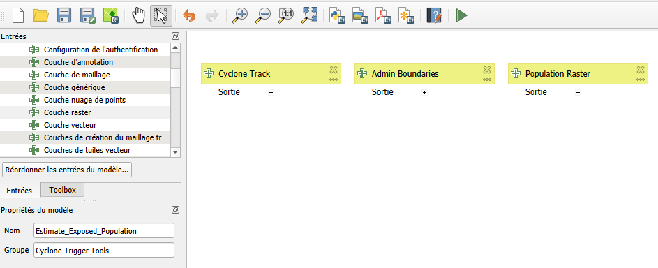
Add model inputs:
On the left panel, expand the Inputs section.
Add the following input layers with type constraints:
+ Vector LayerLabel:
Cyclone TrackIn the Advanced panel, set geometry type to
Line
+ Raster LayerLabel:
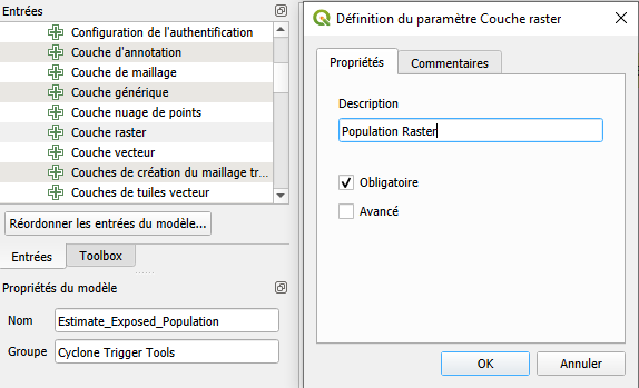
Population Raster
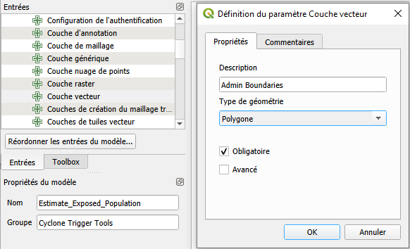
+ Vector LayerLabel:
Admin BoundariesIn the Advanced panel, set geometry type to
Polygon
These will appear at the top of your model canvas and serve as the input data when the model is run.
Tip
All inputs should be set as mandatory, so the model always receives the necessary data to run correctly.

Definition of the model input: Cyclon Track#
Definition of the model input: Admin Bounderies#
Definition of the model input: Population Raster#
Intermediate Result
Résultat intermédiaire de la définition des données d’entrée du modèle#
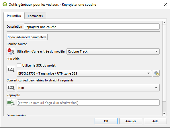
Reproject the cyclone track to EPSG:29738
From the Algorithms panel, search for Reproject Layer .
In the configuration window:
Add a description:
Reprojecter la couche de trajectoire du cyclone a EPSG : 29738Set Input layer to
Cyclone Track(from Model Input).Set Target CRS to
EPSG:29738 – Madagascar / Laborde Grid.Set the output to Model Output (leave the output name empty).
Click OK to add the step to the model.
Reprojecter la couche de trajectoire du cyclone vers un système de référence de coordonnées métrique (CRS) EPSG : 29738#
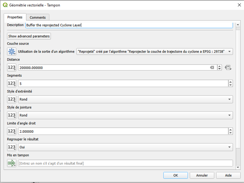
Buffer the reprojected cyclone track
From the Algorithms panel, search for Buffer.
In the configuration window:
Add a description:
Mettre en mémoire tampon la couche Cyclone reprojetéeAdd a description:
Set Input layer to the output from the previous step (from Algorithm Output).
Set Distance to
200000(200 km).Leave Segments at the default value (
5).Set Dissolve result to
Yes.Set the output to Model Output (leave the output name empty).
Click OK to add the step to the model.
Mettre en mémoire tampon la couche Cyclone reprojetée#
Reproject the buffer back to EPSG:4326
From the Algorithms panel, search for Reproject Layer.
In the configuration window:
Add a description:
Reprojecter le tampon vers EPSG:4326In the configuration window:
Set Input layer to the output from the previous step (from Algorithm Output).
Set Target CRS to
EPSG:4326 – WGS 84.Set the output to Model Output (leave the output name empty).
Click OK to add the step to the model.
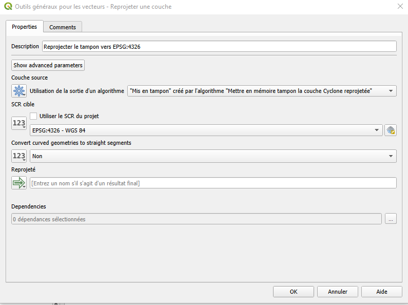
Reprojecter le tampon vers EPSG:4326#
Clip the population raster using the buffered area
From the Algorithms panel, search for Clip Raster by Mask Layer .
In the configuration window:
Add a description:
Découper la couche raster de population pour l'étendre au tampon Cyclon
In the configuration window:
Set Input layer to
Population Raster(from Model Input).Set Mask layer to the output from the previous step (from Algorithm Output).
Set the output to Model Output (leave the output name empty).
Click OK to add the step to the model.
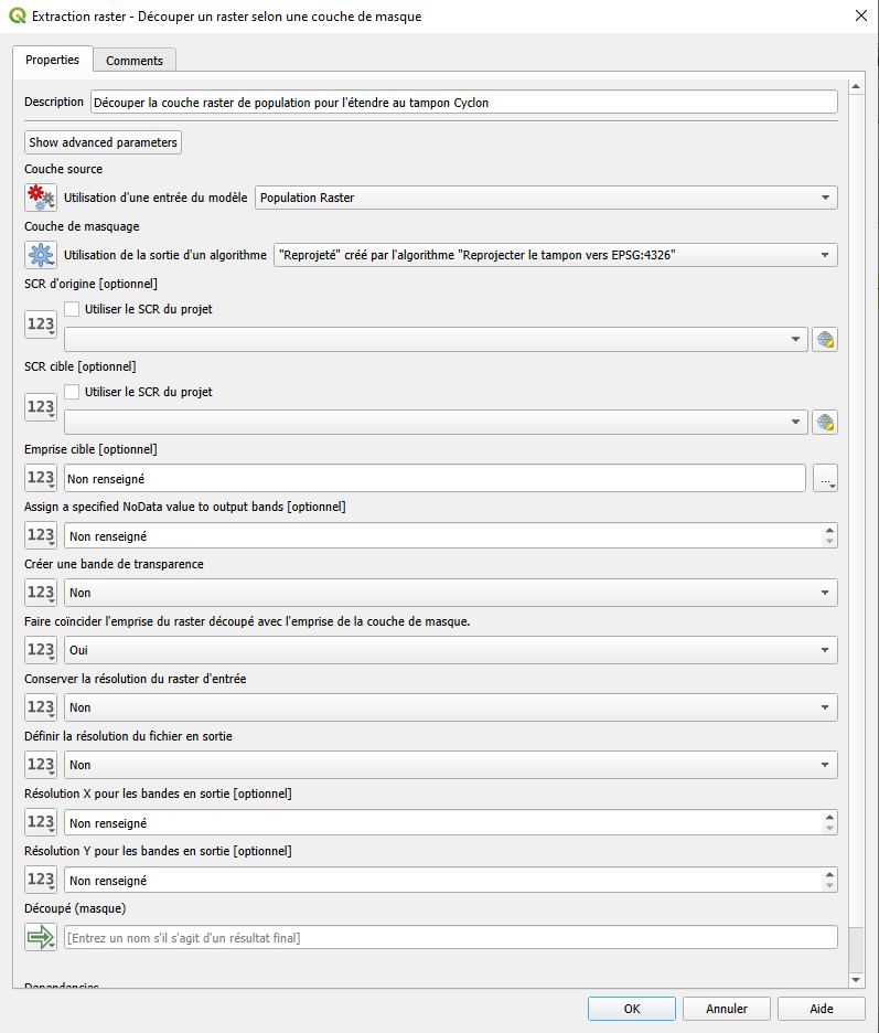
Découper la couche raster de population pour l’étendre au tampon Cyclon#
Calculate zonal statistics to estimate exposed population
From the Algorithms panel, search for Zonal Statistics .
In the configuration window: Calcul de la population exposée aux cyclones par district
Add a description:
Calcul de la population exposée aux cyclones par districtSet Input layer to
Admin Boundaries(from Model Input).Set Raster layer to the output of the previous step (from Algorithm Output).
Set Output column prefix to
exposed_population_.Under Statistics to calculate, select
Sum.Set the output to Model Output and name it:
exposed_population_sumClick
OKto add the step to the model.
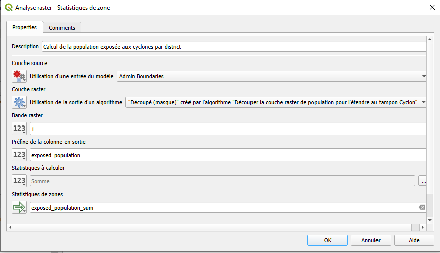
Calcul de la population exposée aux cyclones par district#
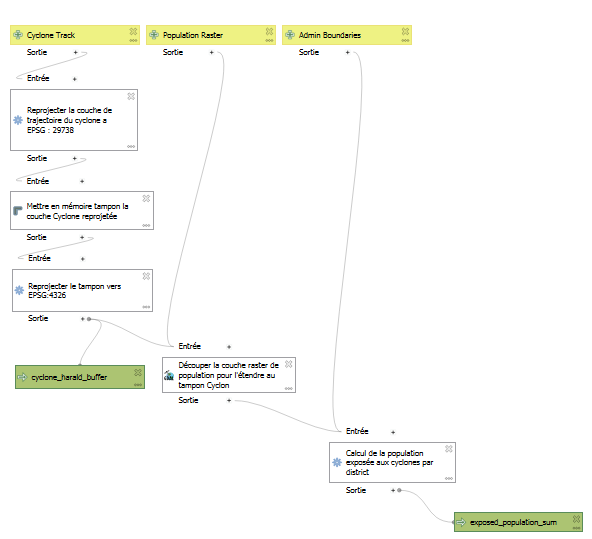
Your results should look something like this:
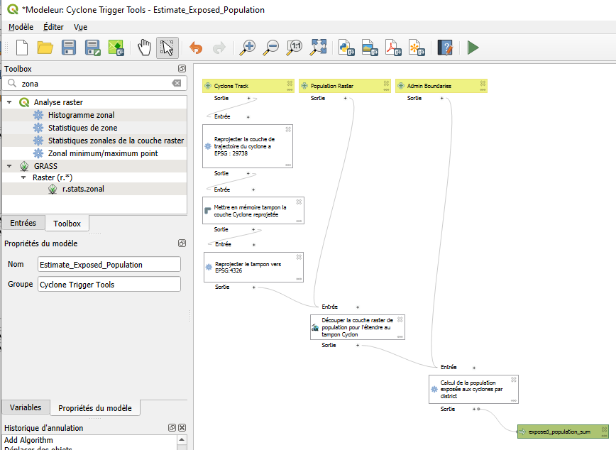
Votre modèle devrait ressembler à ceci. Tous les algorithmes sont correctement connectés et la sortie du modèle est définie.#
Validate your model (recommended)
Before saving or running, click the ✔️ Validate Model button in the top toolbar.
Fix any warnings or errors shown in the log panel.
This helps ensure your model is complete and won’t break during execution.
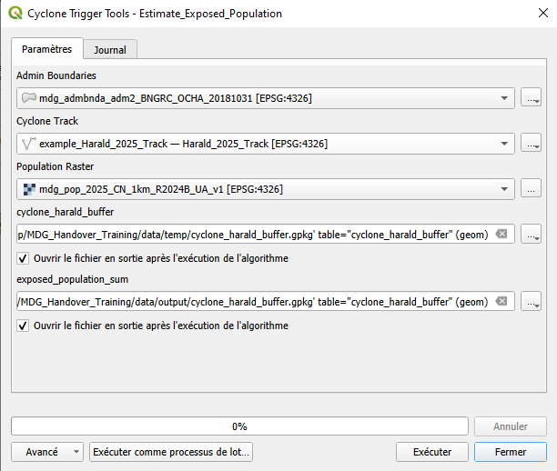
Run the model
Run the model by clicking on
Model->Run ModelSet Admin Bounderies to
mdg_admbnda_adm2_BNGRC_OCHA_20181031.gpkgSet Cyclone Track to
example_Harald_2025_TrackSet Population Raster to
MDG_WorldPop_2020_constrained.tifSet the model output exposed_population_sum to
Harald_Exposed_Populationand save it in thedata->output
You can now run this model any time a new cyclone track becomes available.
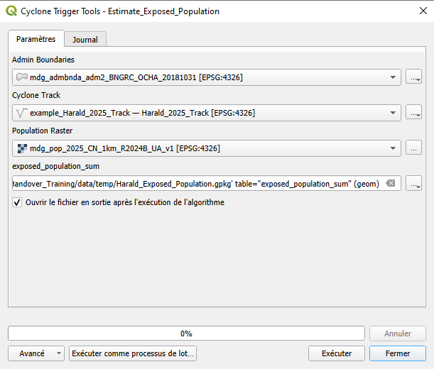
Pour exécuter le modèle, spécifiez l’entrée comme indiqué dans l’image et définissez le nom de la couche de sortie.#
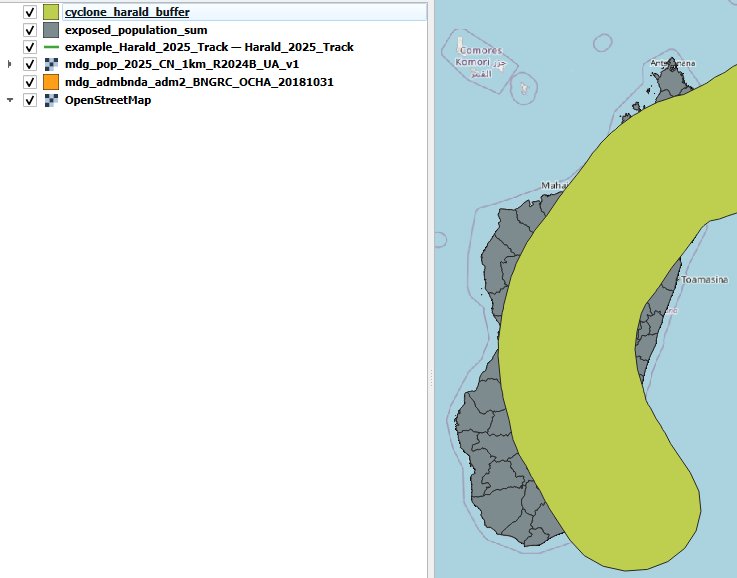
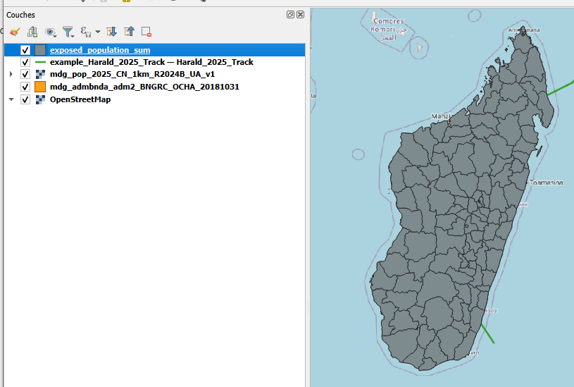
Your results should look something like this:
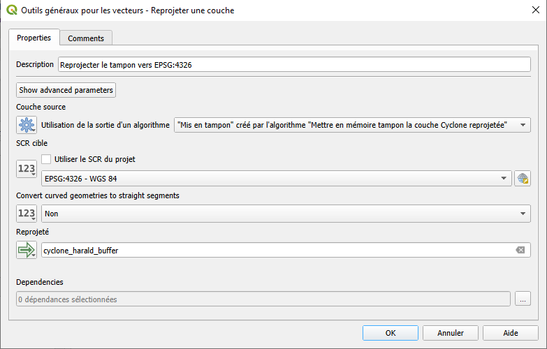
Add the cyclone buffer as an additional model output
Double-click on the algorithm from step 7 (Reproject the buffer back to EPSG:4326) to open its configuration.
In the Output layer field, check the box for Model Output.
Give the output a clear name, for example:
cyclone_harald_bufferClick OK to save the change.
This will allow the model to produce both the exposed population results and the buffered cyclone impact zone when it is run.
Run the model again
Run the model by clicking on
Model->Run ModelSet Admin Bounderies to
mdg_admbnda_adm2_BNGRC_OCHA_20181031.gpkgSet Cyclone Track to
example_Harald_2025_TrackSet Population Raster to
MDG_WorldPop_2020_constrained.tifSet the model output cyclone_harald_buffer to
cyclone_harald_bufferand save it in thedata->outputSet the model output exposed_population_sum to
Harald_Exposed_Populationand save it in thedata->output