Exercises 1: Automatisation

🚧This part of training platform is under ⚠️construction⚠️ and may not be shared or published! 🚧

Characteristics of the exercise

Type of trainings exercise:

• This exercise can be used in online and presence training.

• It can be done as a follow-along exercise or individually as a self-study.

Estimated time demand for the exercise

Relevant Wiki Articles

• Zonal Statistics

• Intersection

• Projections

• Buffer

• Clip

• Automatisation

Aim of the exercise: Aina, the GIS expert at the Malagasy Red Cross (CRM), is preparing for the upcoming cyclone season. She wants to improve her team’s ability to act quickly once a storm is forecasted by automating key analyses in QGIS. These include estimating exposed populations, identifying impacted services like health and education, and assessing whether health posts can be reached from key warehouses within a critical 10-hour window. The goal is to prepare an end-to-end analysis and visualization workflow that can support fast, data-driven anticipatory action before a cyclone makes landfall.

Instructions for the trainers

Trainers Corner

Prepare the training

• Take the time to familiarise yourself with the exercise and the provided material.

• Prepare a white-board. It can be either a physical whiteboard, a flip-chart, or a digital whiteboard (e.g. Miro board) where the participants can add their findings and questions.

• Before starting the exercise, make sure everybody has installed QGIS and has downloaded and unzipped the data folder.

• Check out How to do trainings? for some general tips on training conduction

Conduct the training

Introduction:

• Introduce the idea and aim of the exercise.

• Provide the download link and make sure everybody has unzipped the folder before beginning the tasks.

Follow-along:

• Show and explain each step yourself at least twice and slow enough so everybody can see what you are doing, and follow along in their own QGIS-project.

• Make sure that everybody is following along and doing the steps themselves by periodically asking if anybody needs help or if everybody is still following.

• Be open and patient to every question or problem that might come up. Your participants are essentially multitasking by paying attention to your instructions and orienting themselves in their own QGIS-project.

Wrap up:

• Leave time for any issues or questions concerning the tasks at the end of the exercise.

• Leave some time for open questions.

Available Data

Download all datasets here, save the folder on your computer and unzip the file.

The folder is called “ and contains the whole standard folder structure with all data in the input folder and the additional documentation in the documentation folder.

Dataset	Source	Descriptions
Administrative Boundaries	HDX	The administrative boundaries on level 0-4 for Madagascar can be accessed via HDX provided by OCHA. For this trigger mechanism we provide the administrative boundaries on level 1 (regional level) and 2 (district level) as a shapefile.
Cyclone Tracks	International Best Track Archive for Climate Stewardship (IBTrACS)	IBTrACS project is the most complete global collection of tropical cyclones available. It merges recent and historical tropical cyclone data from multiple agencies to create a unified, publicly available, best-track dataset that improves inter-agency comparisons.
education facilities and health sites	HOT Export Tool	The POI data (education facilities and health sites) is downloaded using the HOT Export Tool based on OpenStreetMap data.
Population	WorldPop	The worldpop dataset in raster format provides the estimated total number of people per grid-cell for the year 2020. We will be working with the Constrained Individual countries 2020 dataset at a resolution of 100m.

Context

Aina is the GIS expert at the Croix-Rouge Malagasy (CRM). With the cyclone season approaching, she knows that time is of the essence once a storm is forecasted. Every hour counts when it comes to protecting communities at risk.

This year, Aina wants to be one step ahead. Instead of manually analyzing cyclone data under pressure, she decides to prepare an automated QGIS model that will help her respond quickly and efficiently.

Her goal:

Build a workflow that automatically estimates exposed populations and infrastructure at risk.

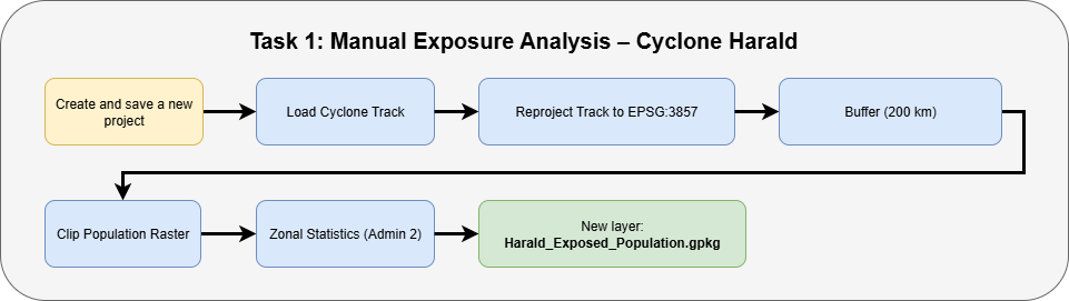
Task 1: Estimating Exposed Population – Aina’s Manual Approach

Before developing the automated model, Aina used to estimate the exposed population manually whenever a cyclone approached Madagascar. In this task, you will follow the steps she used in the past by working with the historical track of Cyclone Harald, WorldPop raster data, and administrative boundaries.

You will manually buffer the cyclone track, clip the population raster, and calculate exposed population using zonal statistics.

1. Open QGIS and create a new project by clicking on Project -> New

2. Save the project in the “project” folder. To do that click on Project -> Save as and navigate to the folder. Name the project “Cyclon_Harald_Exposure”.

3. Load the GeoJOSN file “example_Harald_2025_Track.geojson” in your project by drag and drop (Wiki Video) . Open the folder data -> input

4. Reproject the cyclone track to use meters instead of degrees (important for accurate buffering):

   • In the Processing Toolbox, search for Reproject Layer.

   • Input: example_Harald_2025_Track

   • Target CRS: EPSG:29738 or another meter-based CRS appropriate for Madagascar.

   • Save the result in the temp folder as: Harald_Track_Reprojected

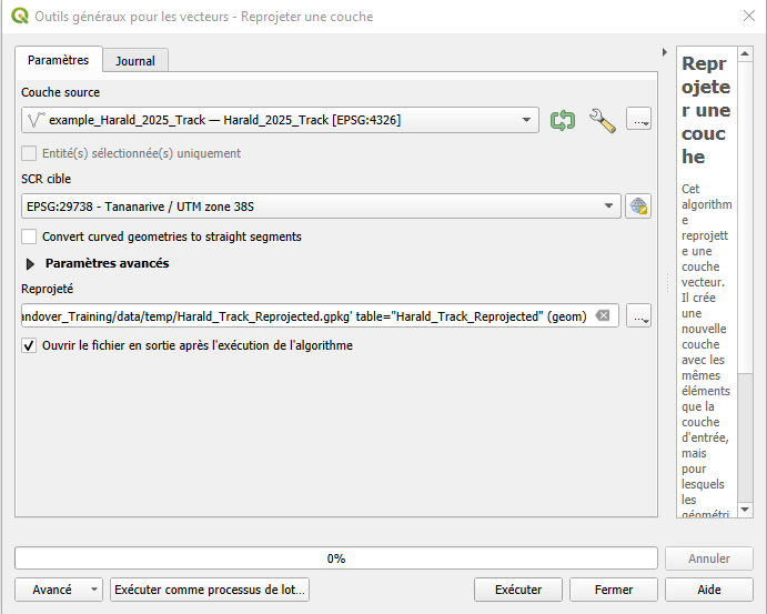
Reprojetter la trajectoire du cyclone

Attention

Buffer distances must be calculated in meters. Many datasets (like GeoJSON cyclone tracks) use geographic coordinate systems like EPSG:4326, which measure in degrees — not meters. To correctly calculate a 200 km buffer, we must first reproject the track into a projected CRS that uses meters.

5. Buffer the cyclone track:

   • In the Processing Toolbox, search for Buffer.

   • Input: Harald_Track_Reprojected

   • Buffer distance: 200000 (meters)

   • Segments: Leave default (5)

   • Dissolve: Yes

   • Save output in the temp folder as: Harald_Buffer_200km

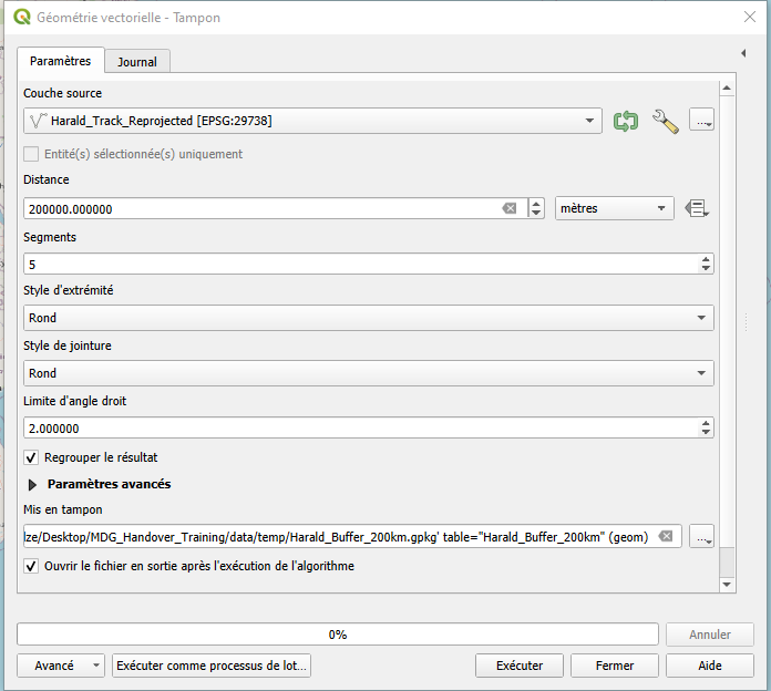
Tamponner la trajectoire du cyclone

Intermediate Result: Buffer

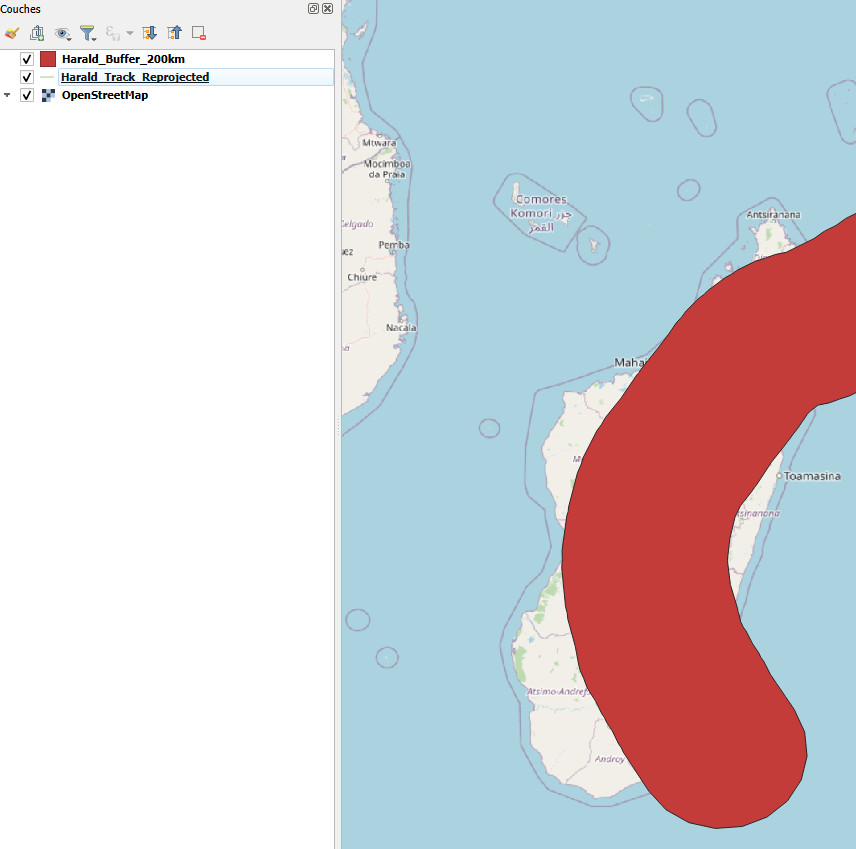
Les résultats intermédiaires doivent montrer la trajectoire du cyclone et la zone tampon de 200 kilomètres autour de celui-ci. La zone tampon doit être une seule entité.

6. Reproject the buffer back to EPSG:4326 (to match the raster’s CRS):

   • In the Processing Toolbox, search for Reproject Layer.

   • Input: Harald_Buffer_200km_29738

   • Target CRS: EPSG:4326 – WGS 84

   • Save the output in the temp folder as: Harald_Buffer_200km_4326

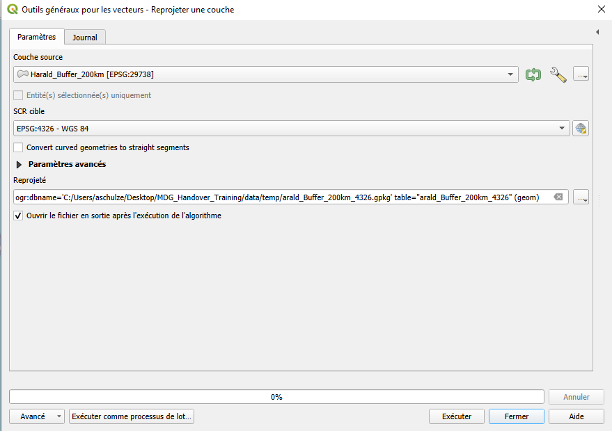
Reprojetter la tamponner trajectoire du cyclone

7. Load the administrative boundaries:

   • File: mdg_admbnda_adm2_BNGRC_OCHA_20181031.gpkg

   • Add using drag and drop or Add Vector Layer.

8. Load the population raster:

   • File: MDG_WorldPop_2020_constrained.tif

   • Add using Layer → Add Raster Layer.

9. Clip the population raster using the buffered impact zone:

   • In the Processing Toolbox, search for Clip Raster by Mask Layer.

   • Input raster: MDG_WorldPop_2020_constrained

   • Mask layer: Harald_Buffer_200km

   • Save output in the temp folder as: Harald_Pop_Clip

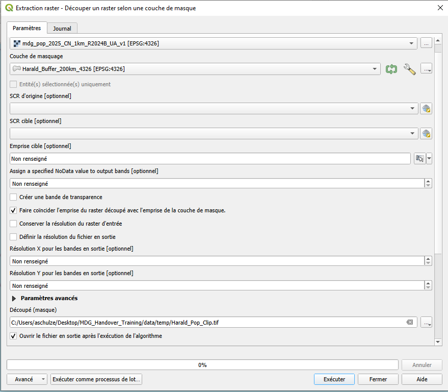
Découpez la population ratser selon la zone affectée par le cyclone (trajectoire tampon du cyclone)

Intermediate Result: Clip Population Raster Alyer

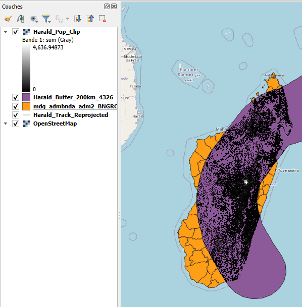
Résultat intermédiaire du découpage de la couche raster de population à l’étendue de la trajectoire tamponnée du cyclone.

10. Calculate total exposed population:

• In the Processing Toolbox, search for Zonal Statistics.

• Input vector layer: mdg_admbnda_adm2_BNGRC_OCHA_20181031.gpkg

• Raster layer: Harald_Pop_Clip

• Statistic to calculate: Sum

• Field prefix: e.g., exposed_population_

• Save the updated vector layer in the result folder as: Harald_Exposed_Populationg

• The result will be a new column in the attribute table of the mdg_admbnda_adm2_BNGRC_OCHA_201810312.gpkg layer, showing the total population within the cyclone buffer per district.

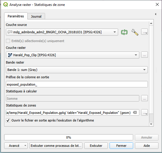
Calcul de la population exposée aux cyclones par district sur la base du raster de population.

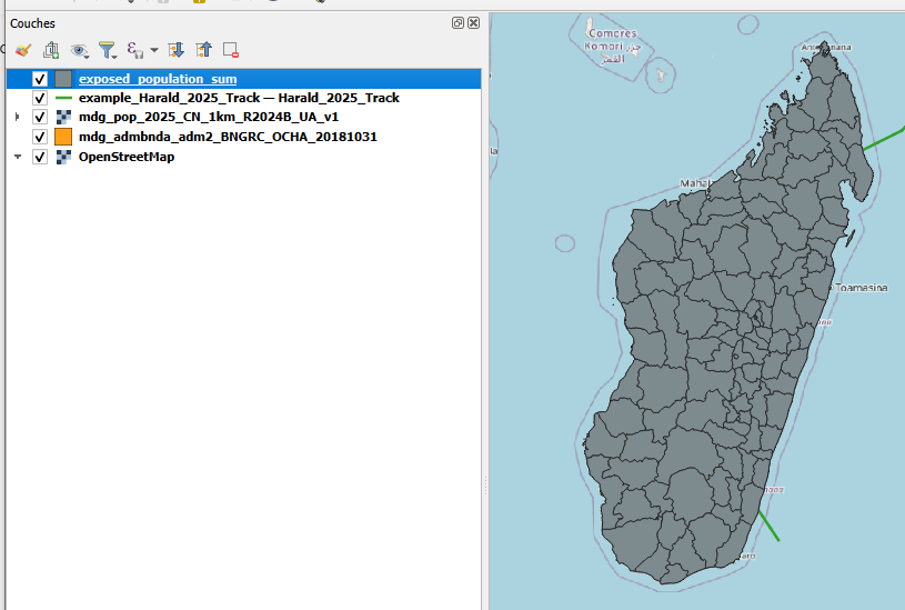
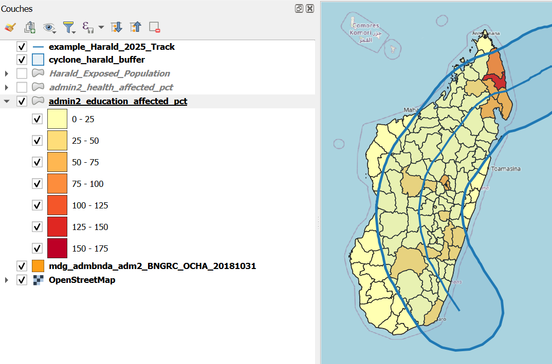
11. Visualise the affected population by classifying the results: Now that Aina has estimated the exposed population in each district, she wants to clearly show the differences across regions on the map. To do this, we’ll apply a graduated classification to the Harald_Exposed_Population layer using the new population field created by the Zonal Statistics tool.

• In the Layers panel, right-click on the layer Harald_Exposed_Population and choose Properties.

• Go to the Symbology tab on the left.

• At the top of the window, change the style from Single Symbol to Graduated.

• In the Value drop-down menu, select the field that contains the population sum. It typically starts with the prefix you defined earlier, e.g. exposed_population_sum.

• Set the color ramp to one that suits your map (e.g. Reds).

• Choose a classification mode (e.g. Quantile, Natural Breaks, or Equal Interval) and select the number of classes (e.g. 5).

• Click Classify to generate the classification.

• Click Apply and then OK to display the classified map.

Tip

You can adjust class boundaries or labels by double-clicking on each class entry.

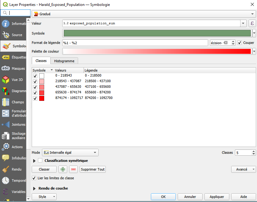
Configuration of the visualisation of the exposed population in five classes.

Your results should look something like this:

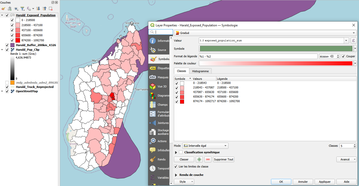
Visualisation de la population exposée en cinq classes.

Task 2: Automation of Exposed Population Estimation – Aina’s Model

After manually estimating exposed populations in past cyclone seasons, Aina has decided to prepare an automated model using the QGIS Graphical Modeller. This will help her move faster and avoid repeating the same steps manually each time a cyclone is forecasted.

In this task, you will help Aina build a simple version of that model using the tools from Task 1. The model should:

• Reproject the cyclone track to EPSG:29738

• Buffer the cyclone track

• Reproject the buffer back to EPSG:4326

• Clip the population raster

• Run Zonal Statistics to get exposed population per district

---

1. Set up the model structure:

   • Open the Graphical Modeler from the top menu:
     Processing → Graphical Modeler…

2. Naming the model:

   • A new model window will open. On the left side, click on Model Properties to define basic information about the model:

     • Model Name: Estimate_Exposed_Population

     • Group: Cyclone Trigger Tools

     • Leave the description empty or write: “Automated model to estimate exposed population based on cyclone buffer.”

3. Save the model

   • To save the model:

     • Click the Save icon (💾) or go to Model → Save.

     • Navigate to the models folder of your training structure.

     • Save the model as:
       Estimate_Exposed_Population

4. Add model inputs:

   • On the left panel, expand the Inputs section.

   • Add the following input layers with type constraints:

     • + Vector Layer

       • Label: Cyclone Track

       • In the Advanced panel, set geometry type to Line

     • + Raster Layer

       • Label: Population Raster

     • + Vector Layer

       • Label: Admin Boundaries

       • In the Advanced panel, set geometry type to Polygon

   • These will appear at the top of your model canvas and serve as the input data when the model is run.

     Tip

     All inputs should be set as mandatory, so the model always receives the necessary data to run correctly.

Input Cyclon Track

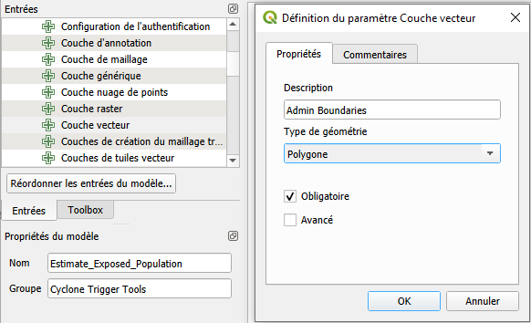
Definition of the model input: Cyclon Track

Input Admin Boundaries

Definition of the model input: Admin Bounderies

Population Raster

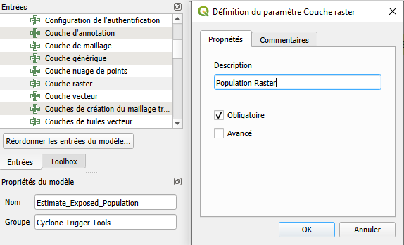
Definition of the model input: Population Raster

Intermediate Result

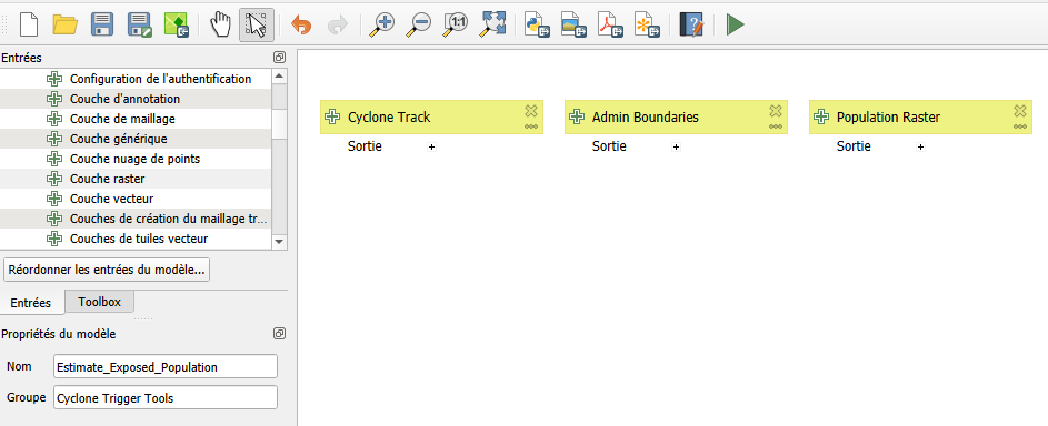
Résultat intermédiaire de la définition des données d’entrée du modèle

5. Reproject the cyclone track to EPSG:29738

   • From the Algorithms panel, search for Reproject Layer .

   • In the configuration window:

     • Add a description: Reprojecter la couche de trajectoire du cyclone a EPSG : 29738

     • Set Input layer to Cyclone Track (from Model Input).

     • Set Target CRS to EPSG:29738 – Madagascar / Laborde Grid.

     • Set the output to Model Output (leave the output name empty).

   • Click OK to add the step to the model.

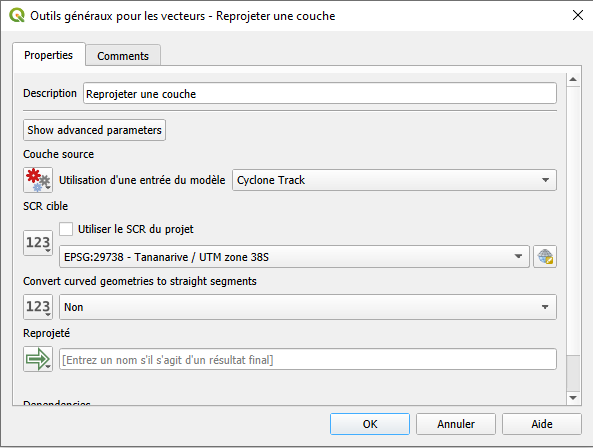
Reprojecter la couche de trajectoire du cyclone vers un système de référence de coordonnées métrique (CRS) EPSG : 29738

6. Buffer the reprojected cyclone track

   • From the Algorithms panel, search for Buffer.

   • In the configuration window:

   • Add a description: Mettre en mémoire tampon la couche Cyclone reprojetée

   • Add a description:

   • Set Input layer to the output from the previous step (from Algorithm Output).

   • Set Distance to 200000 (200 km).

   • Leave Segments at the default value (5).

   • Set Dissolve result to Yes.

   • Set the output to Model Output (leave the output name empty).

   • Click OK to add the step to the model.

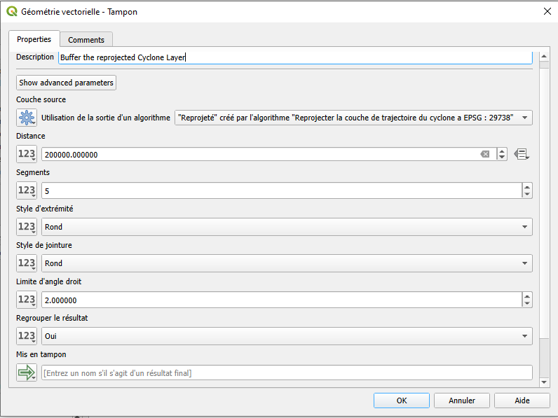
Mettre en mémoire tampon la couche Cyclone reprojetée

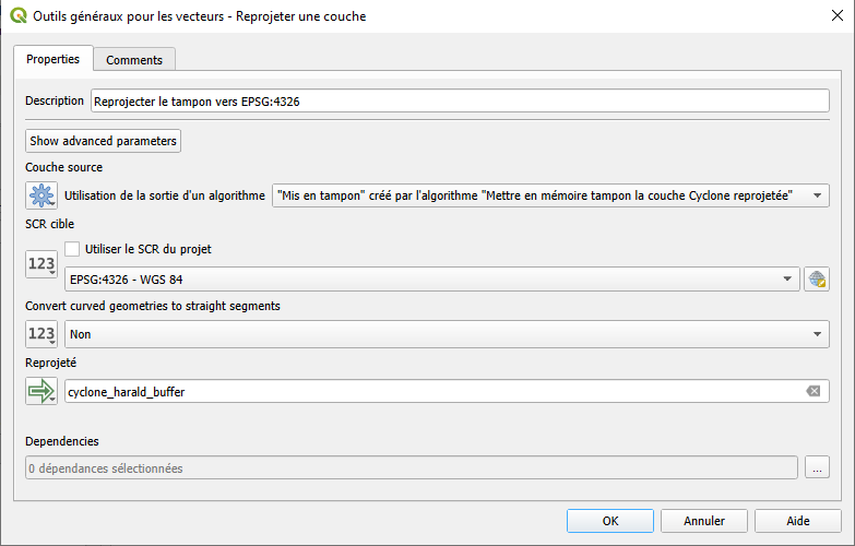
7. Reproject the buffer back to EPSG:4326

   • From the Algorithms panel, search for Reproject Layer.

   • In the configuration window:

   • Add a description: Reprojecter le tampon vers EPSG:4326

   • In the configuration window:

     • Set Input layer to the output from the previous step (from Algorithm Output).

     • Set Target CRS to EPSG:4326 – WGS 84.

     • Set the output to Model Output (leave the output name empty).

   • Click OK to add the step to the model.

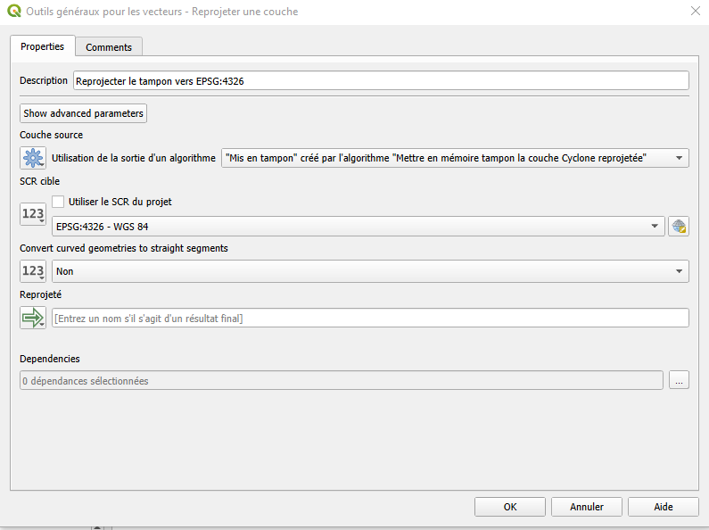
Reprojecter le tampon vers EPSG:4326

8. Clip the population raster using the buffered area

   • From the Algorithms panel, search for Clip Raster by Mask Layer .

   • In the configuration window:

     • Add a description: Découper la couche raster de population pour l'étendre au tampon Cyclon

   • In the configuration window:

     • Set Input layer to Population Raster (from Model Input).

     • Set Mask layer to the output from the previous step (from Algorithm Output).

     • Set the output to Model Output (leave the output name empty).

   • Click OK to add the step to the model.

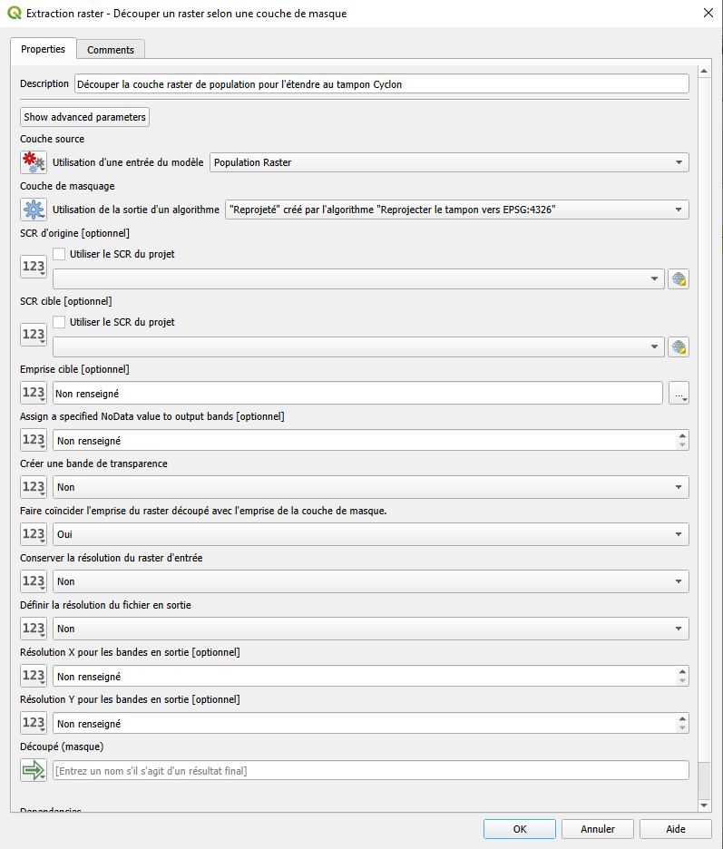
Découper la couche raster de population pour l’étendre au tampon Cyclon

9. Calculate zonal statistics to estimate exposed population

   • From the Algorithms panel, search for Zonal Statistics .

   • In the configuration window: Calcul de la population exposée aux cyclones par district

     • Add a description: Calcul de la population exposée aux cyclones par district

     • Set Input layer to Admin Boundaries (from Model Input).

     • Set Raster layer to the output of the previous step (from Algorithm Output).

     • Set Output column prefix to exposed_population_.

     • Under Statistics to calculate, select Sum.

     • Set the output to Model Output and name it:

     exposed_population_sum
     

   • Click OK to add the step to the model.

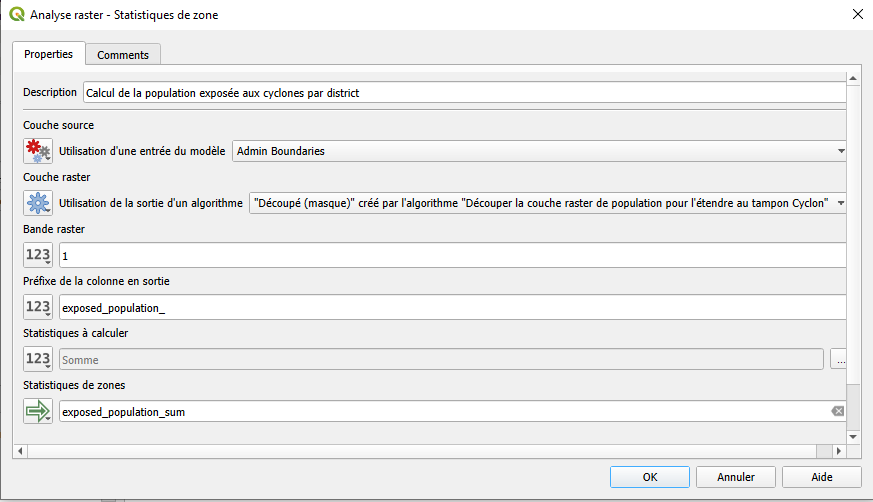
Calcul de la population exposée aux cyclones par district

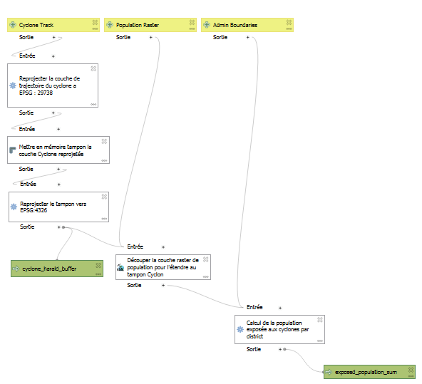
Your results should look something like this:

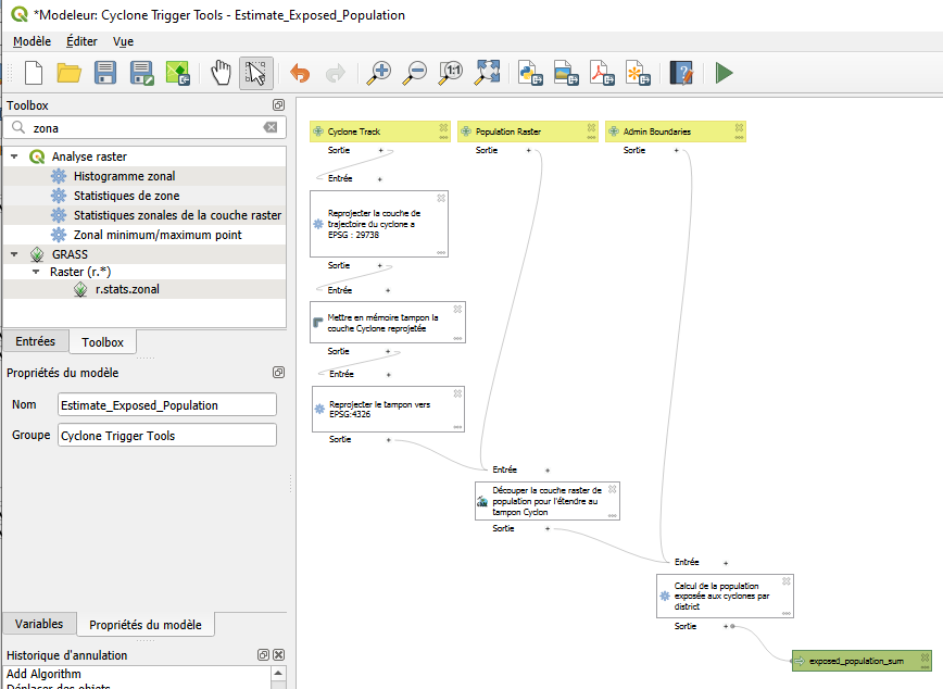
Votre modèle devrait ressembler à ceci. Tous les algorithmes sont correctement connectés et la sortie du modèle est définie.

10. Validate your model (recommended)

• Before saving or running, click the ✔️ Validate Model button in the top toolbar.

• Fix any warnings or errors shown in the log panel.

• This helps ensure your model is complete and won’t break during execution.

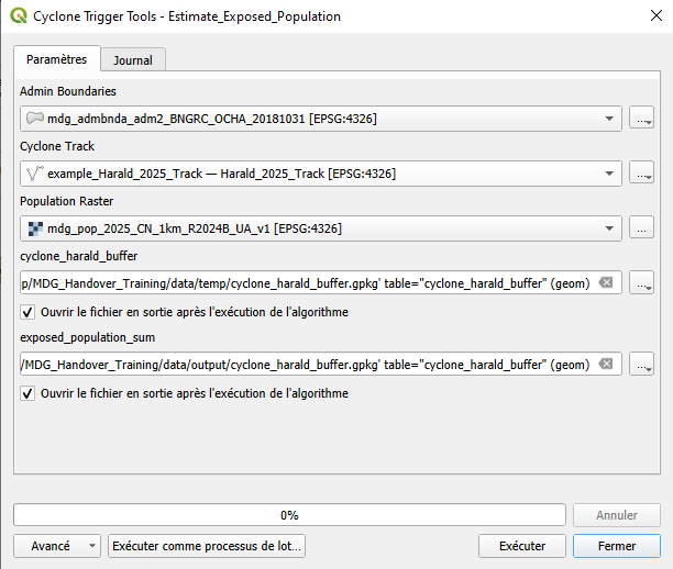
11. Run the model

• Run the model by clicking on Model -> Run Model

• Set Admin Bounderies to mdg_admbnda_adm2_BNGRC_OCHA_20181031.gpkg

• Set Cyclone Track to example_Harald_2025_Track

• Set Population Raster to MDG_WorldPop_2020_constrained.tif

• Set the model output exposed_population_sum to Harald_Exposed_Populationand save it in the data -> output

You can now run this model any time a new cyclone track becomes available.

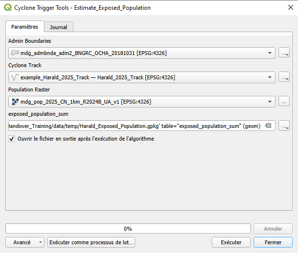
Pour exécuter le modèle, spécifiez l’entrée comme indiqué dans l’image et définissez le nom de la couche de sortie.

Your results should look something like this:

12. Add the cyclone buffer as an additional model output

• Double-click on the algorithm from step 7 (Reproject the buffer back to EPSG:4326) to open its configuration.

• In the Output layer field, check the box for Model Output.

• Give the output a clear name, for example:

  cyclone_harald_buffer
  

• Click OK to save the change.

• This will allow the model to produce both the exposed population results and the buffered cyclone impact zone when it is run.

13. Run the model again

• Run the model by clicking on Model -> Run Model

• Set Admin Bounderies to mdg_admbnda_adm2_BNGRC_OCHA_20181031.gpkg

• Set Cyclone Track to example_Harald_2025_Track

• Set Population Raster to MDG_WorldPop_2020_constrained.tif

• Set the model output cyclone_harald_buffer to cyclone_harald_bufferand save it in the data -> output

• Set the model output exposed_population_sum to Harald_Exposed_Populationand save it in the data -> output

Graphic Modler Output Buffer

Definition of the model input: Admin Bounderies

Run Model with Buffer Output

Definition of the model input: Population Raster

Model Output

Definition of the model input: Population Raster

Task 3: Identifying Affected Health Facilities and Schools – Aina Adds More Layers

After building her model to estimate exposed population, Aina wants to expand its usefulness. She decides to also identify critical services affected by cyclones — especially health facilities and schools.

Not only does she want to know which facilities are affected, but also how many in total exist per district. That way, she can calculate the percentage of services affected in each area.

To achieve this, she will use two point datasets from OpenStreetMap:

• Health facilities

• Education facilities

1. Load the health and education facilities datasets First, let’s have a look at the data we want to work with.

• Navigate to your input data folder.

• Drag and drop the following layers into your QGIS project:

  • hotosm_mdg_health_facilities

  • hotosm_mdg_education_facilities

• Confirm that both layers are visible in the Layers Panel

2. Save your model under a new name

   • Open your existing model Estimate_Exposed_Population.model3.

   • Immediately save it under a new name:

     • Click Model → Save As…

     • Save it to the project folder as:

Estimate_Exposed_Population_Health_Education

3. Add new model inputs

   • In the Inputs section, add:

     • Vector Layer

       • Description:

       Health Facilities
       

       • Set Geometry Type to Point

     • Vector Layer

       • Description:

       Education Facilities
       

       • Set Geometry Type to Point

Model Input: Health Facilities

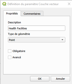
Définir une nouvelle entrée de modèle : couche vectorielle de points représentant les établissements de santé

Model Input: Education Facilities

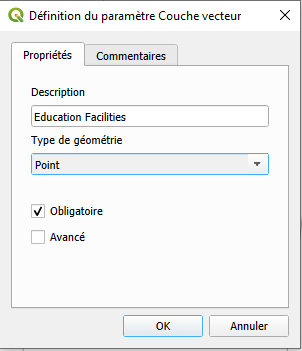
Définir une nouvelle entrée de modèle : couche vectorielle de points représentant les établissements d’enseignement

3. Count All Health Facilities per Admin 2

   • From the Algorithms panel, search for Count Points in Polygon.

   • Configuration:

     • Add a description: Comptez le nombre d'établissements de santé dans chaque district.

     • Polygon layer: Admin Boundaries (Model Input)

     • Points layer: Health Facilities (Model Input)

     • Count field name:

     Count_health_total
     

     • Leave output as Model Output

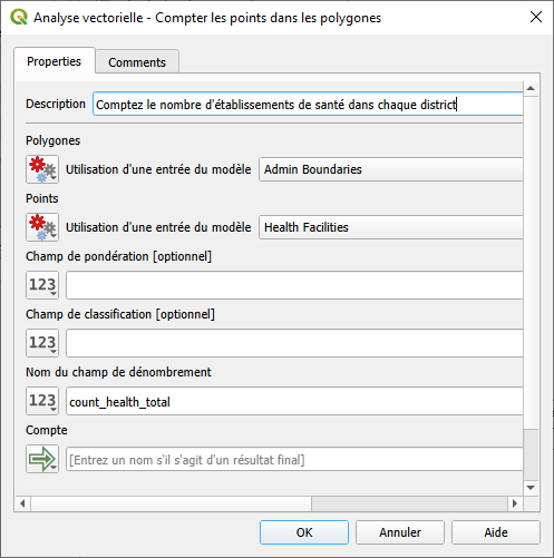
Configuration de l’opération : compter le nombre d’établissements de santé dans chaque district.

4. Count All Education Facilities per Admin 2

   • Add another Count Points in Polygon step.

   • Configuration:

     • Add a description: Comptez le nombre d'établissements de education dans chaque district

     • Polygon layer: Admin Boundaries (Model Input)

     • Points layer: Education Facilities (Model Input)

     • Count field name:

     count_education_total
     

     • Leave output as Model Output

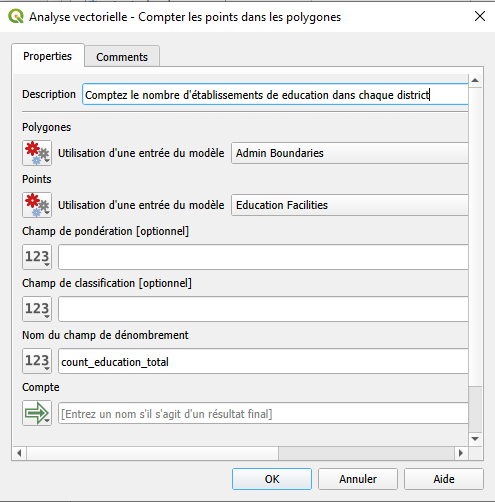
Configuration de l’opération : compter le nombre d’établissements scolaires dans chaque district.

5. Intersect Health Facilities with Cyclone Buffer

   • From the Algorithms panel, search for Intersection.

   • In the configuration window:

   • Add a description:

     Établissements de santé dans la zone d'impact du cyclone
     

     • Input layer: Health Facilities (Model Input)

     • Overlay layer: buffered cyclone zone (use “Reprojected to EPSG:4326” from Algorithm Output)

     • Leave output as Model Output

   • Click OK

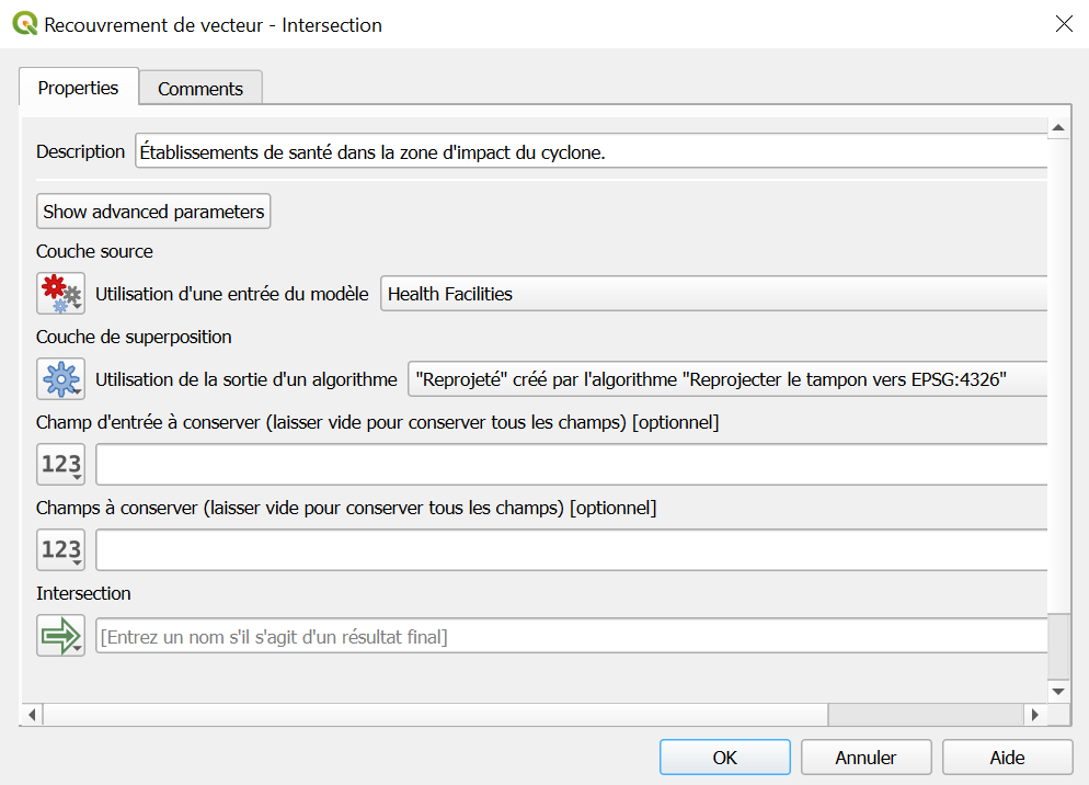
Configuration de l’opération : intersecter les établissements de santé avec la zone d’impact du cyclone.

6. Intersect Education Facilities with Cyclone Buffer

   • Add another Intersection algorithm.

   • Configuration:

     • Add a description:

       Établissements de education dans la zone d'impact du cyclone.
       

     • Input layer: Education Facilities (Model Input)

     • Overlay layer: buffered cyclone zone (use “Reprojected to EPSG:4326” from Algorithm Output)

     • Leave output as Model Output

   • Click OK

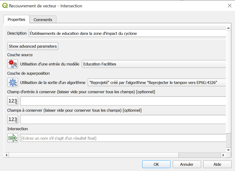
Configuration de l’opération : intersecter les établissements de education avec la zone d’impact du cyclone.

7. Count Affected Health Facilities per Admin 2

   • Add Count Points in Polygon

   • Add a description: Compter les établissements de santé touchés par district

   • Configuration:

     • Add a description: Compter les établissements de santé touchés par district

       Compter les établissements de santé touchés par district
       

     • Polygon layer: Count total health facilities output

     • Points layer: intersected health facilities output

     • Count field name:

       sum_exposed_health
       

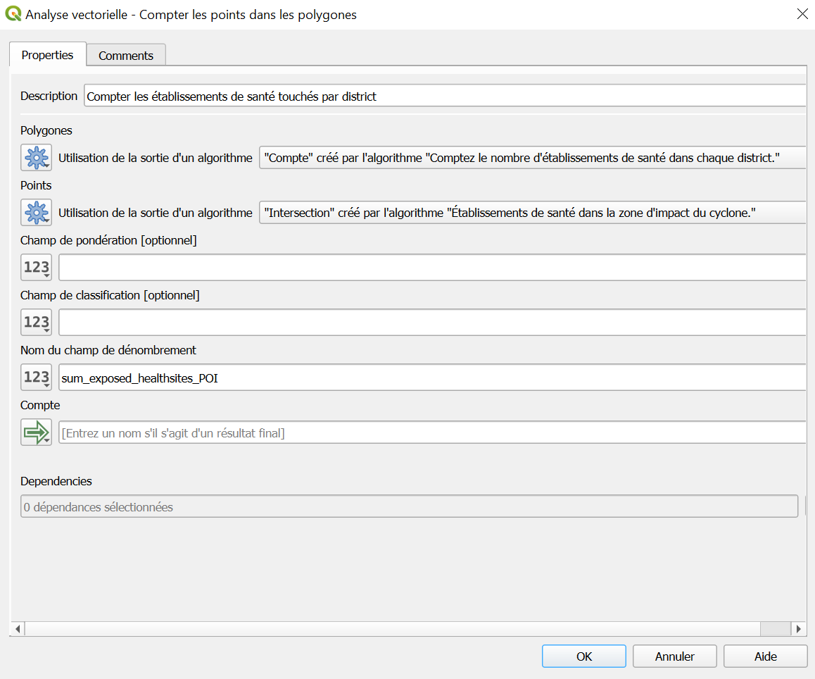
Configuration de l’opération : compter les établissements de santé touchés par district.

8. Count Affected Education Facilities per Admin 2

   • Add Count Points in Polygon

   • Add a description: Compter les établissements education touchés par district

   • Configuration:

     • Add a description:

       Compter les établissements education touchés par district
       

     • Polygon layer: Count total education facilities output

     • Points layer: intersected education facilities output

     • Count field name:

       sum_exposed_education
       

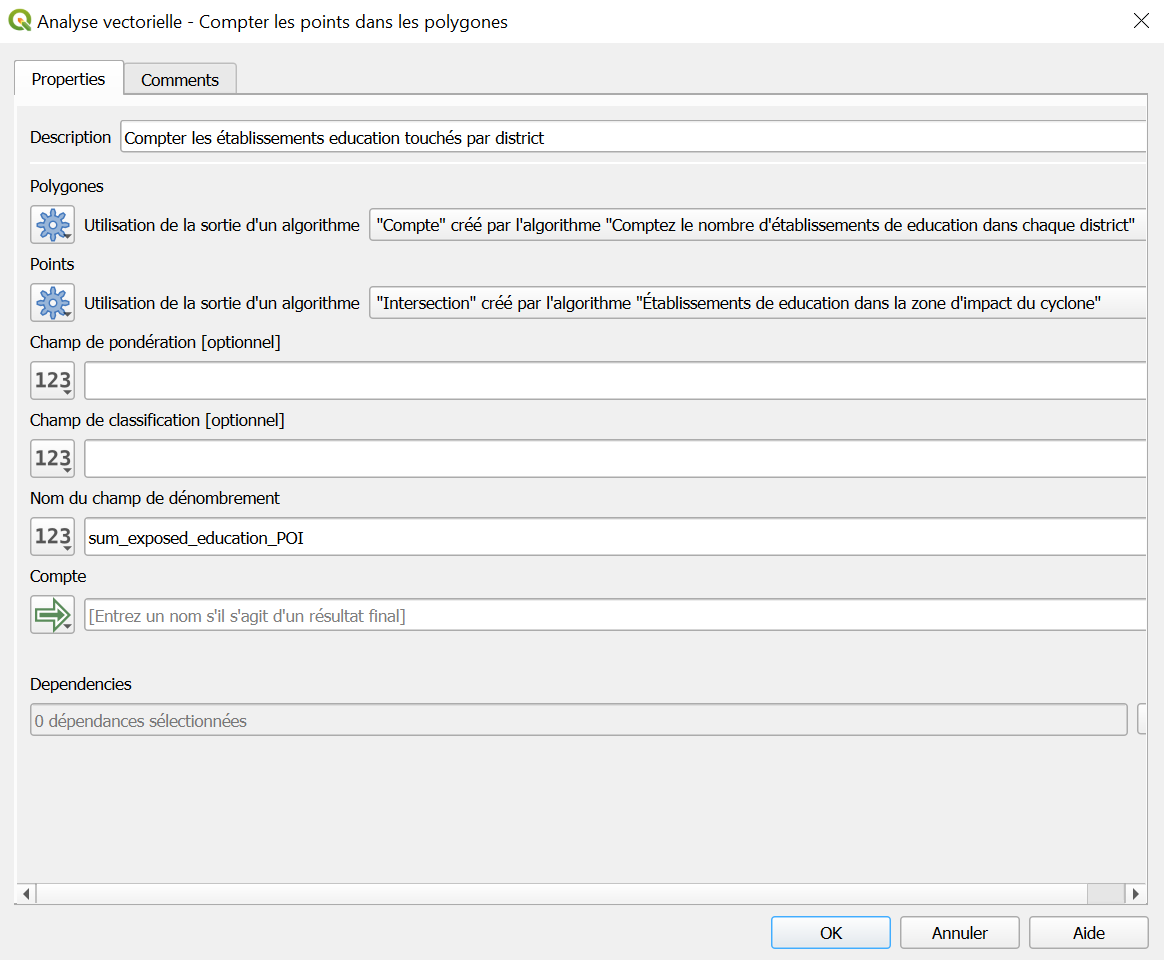
Configuration de l’opération : compter les établissements de santé touchés par district.

9. Calculate percentage of affected Health Facilities To compute the percentage of affected health sites per administrative area, we will use the Field Calculator:

• Add the Field Calculator:

  • Add a description: Calculer le pourcentage d’établissements de santé touchés par district

  • Configuration:

    • Add a description:

      Calculer le pourcentage d’établissements de santé touchés par district
      

  • Input layer: the output of Count Affected Health Facilities per Admin 2

  • Output field name:

    pct_exposed_health
    

  • Field type: Decimal (real)

  • Expression:

   CASE WHEN "count_health_total" > 0
   THEN "sum_exposed_health" / "count_health_total" * 100
   ELSE 0
   END
  

  • Set the output as Model Output

  • Name it:

  admin2_health_affected
  

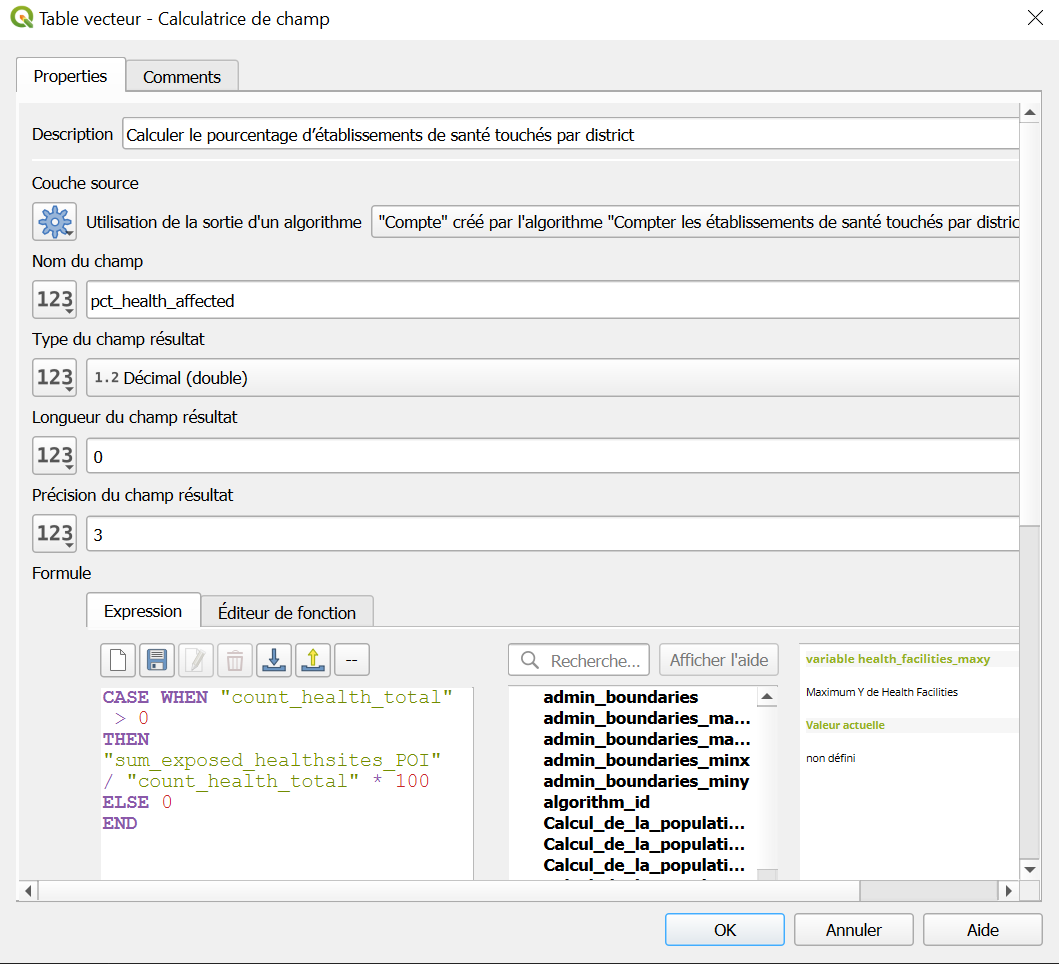
Configuration de l’opération : calculer le pourcentage d’établissements de santé touchés par district.

10. Calculate percentage of affected Education Facilities To compute the percentage of affected education sites per administrative area, we will use the Field Calculator:

• Add the Field Calculator:

  • Add a description: Calculer le pourcentage d’établissements d’éducation touchés par district

  • Configuration:

    • Add a description:

      Calculer le pourcentage d’établissements d’éducation touchés par district
      

    • Input layer: the output of Count Affected Education Facilities per Admin 2

    • Output field name:

      pct_exposed_education
      

    • Field type: Decimal (real)

    • Expression:

      CASE WHEN "count_education_total" > 0
      THEN "sum_exposed_education_POI" / "count_education_total" * 100
      ELSE 0
      END
      

  • Set the output as Model Output

  • Name it:

    admin2_education_affected
    

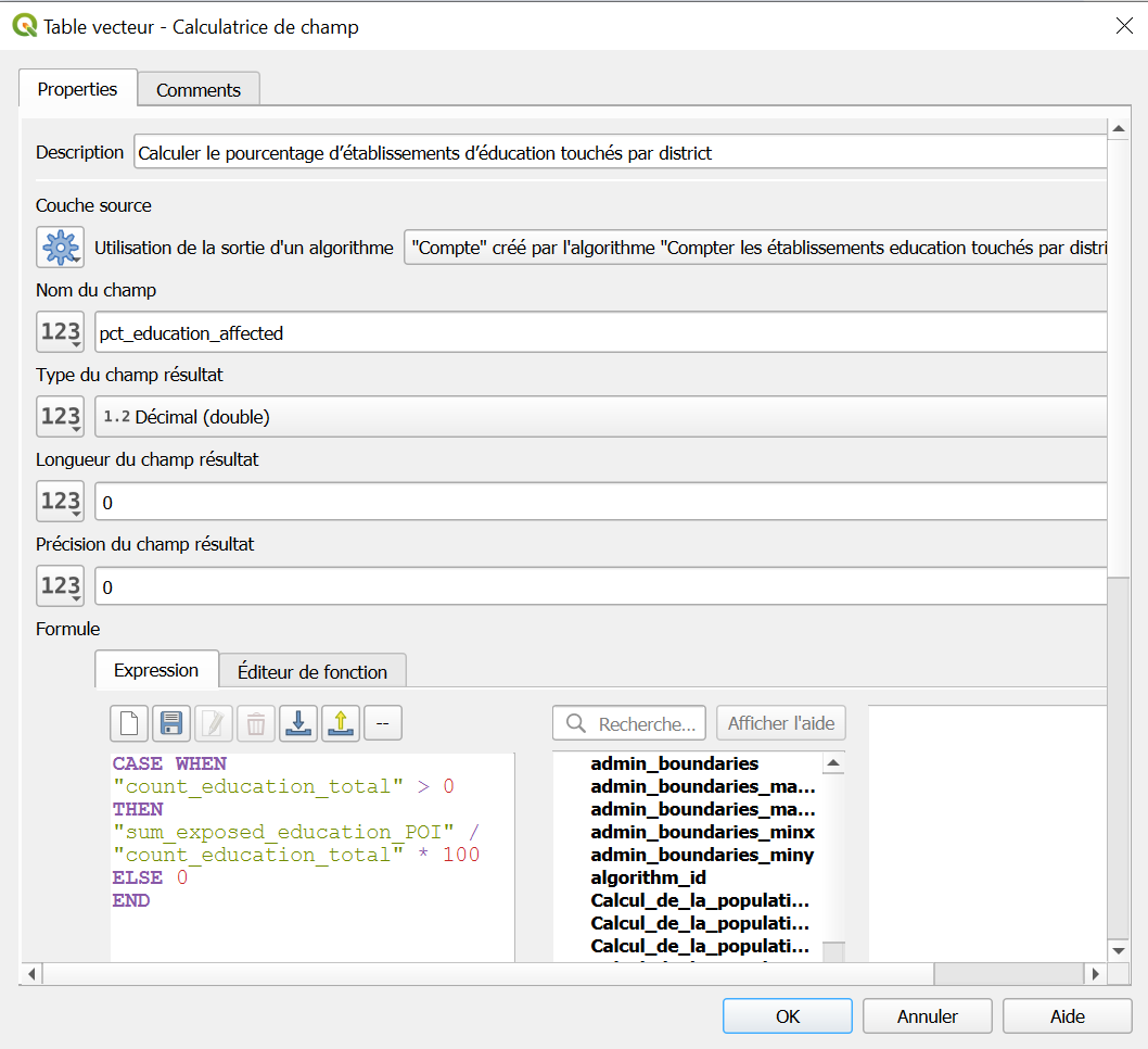
Configuration de l’opération : calculer le pourcentage d’établissements d’éducation touchés par district.

11. Validate and Save Your Extended Model

• Click the ✔️ Validate Model button to check for errors.

• Save again to:
  Estimate_Exposed_Population_Health_Education.model3

12. Run the model

• Click the ▶️ Run button in the top-right corner of the Graphical Modeler window.

• Input:

  • Click on the three dots for each input dataset and select the correct input:

    • Cyclone Track → select the GeoJSON of the storm path (e.g. Harald_2025_Track.geojson)

    • Population Raster → select the WorldPop raster file

    • Admin Boundaries → select the Admin 2 layer (e.g. MDG_adm2.gpkg)

    • Health Facilities → select the point dataset for health sites

    • Education Facilities → select the point dataset for schools

• Output:

  • Save all output layers in the output folder and use the names below.

    • admin2_health_affacted ->

    admin2_health_affected
    

    • admin2_education_affected ->

    admin2_education_affected
    

    • cyclone_harald_buffer ->

    cyclone_harald_buffer
    

    • exposed_population_sum ->

    admin2_harald_Exposed_Population
    

• Click Run to execute the full model.

Graphic Modler

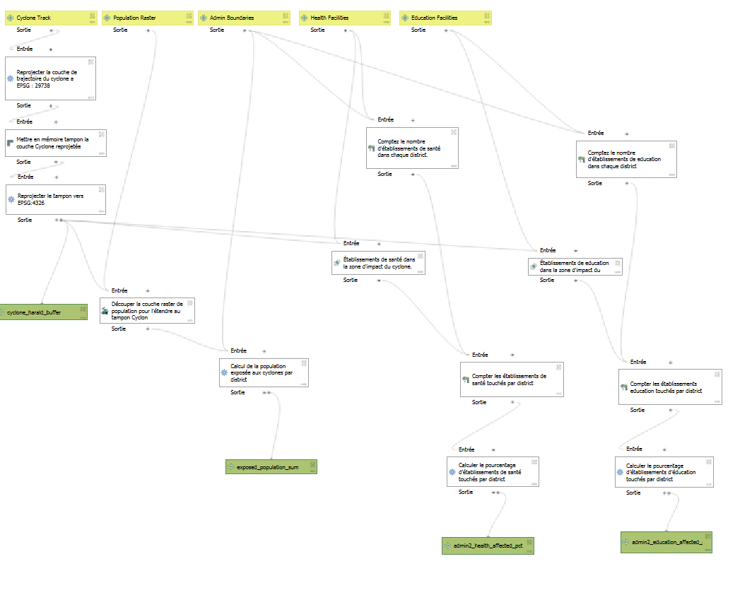
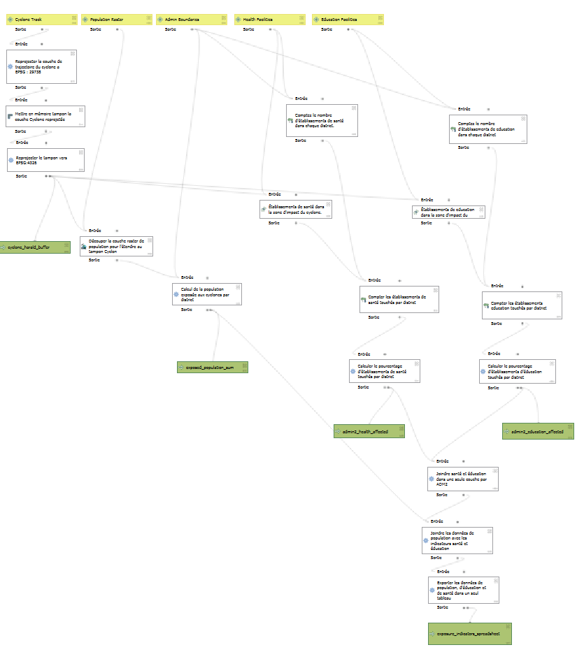
Vue d’ensemble du Modèle Graphique de la tâche 3 montrant tous les algorithmes connectés et les sorties définies.

Run Model Configuration

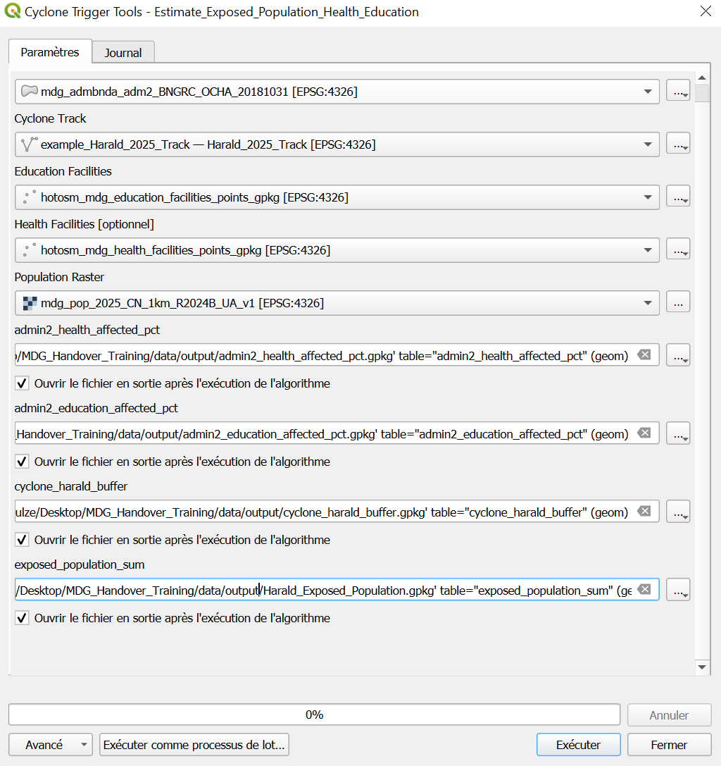
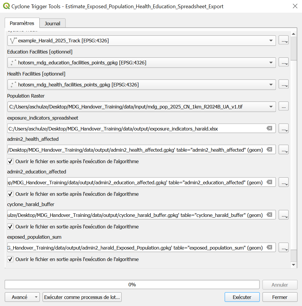
Configuration des paramètres pour exécuter le modèle de la tâche 3 avec toutes les couches d’entrée requises.

Model Output

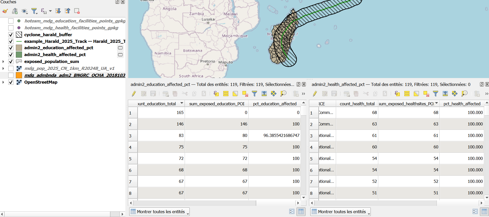
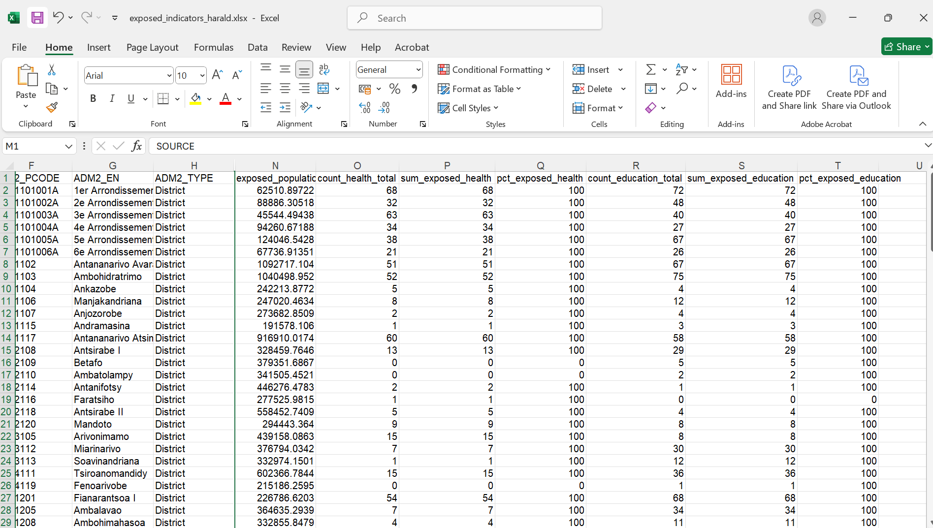
Résultats du modèle de la tâche 3 affichés dans QGIS, y compris les pourcentages d’établissements de santé et d’éducation touchés par district.

---

Task 4: Visualizing Cyclone Impact Results – Aina Styles Her Layers

Aina now has all the analysis results she needs — but numbers and tables alone won’t convince her colleagues or decision-makers. What they need are clear and easy-to-read maps that can be used directly in meetings and reports.

To save time, Aina doesn’t want to adjust colors and legends manually each time a new cyclone comes in. Instead, she will use ready-made style files (.qml) that instantly give layers a professional and consistent look. Where no style exists yet, she will create one herself, so that next time the map can be updated with just a few clicks.

In this task, you will help Aina make her cyclone impact maps both informative and visually compelling by applying and creating QGIS style files.

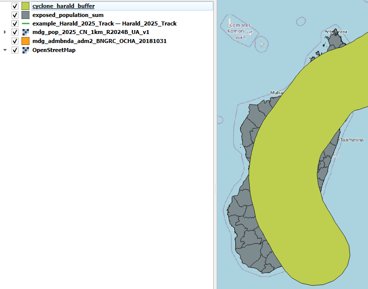
1. Load Required Layers (if not already loaded)

Make sure the following layers are already loaded into your QGIS project. These are outputs from Task 3:

• example_Harald_2025_Track

• cyclone_harald_buffer

• Harald_Exposed_Population

• admin2_health_affected

• admin2_education_affected

If any are missing:

• Load them using drag & drop from your results folder, or

• Use Layer → Add Layer → Add Vector Layer or Add Raster Layer

---

2. Apply Predefined Style Files

Apply the following.qml style files to the respective layers:

Layer	Style File
example_Harald_2025_Track	storm_track_cyclone_style.qml
cyclone_harald_buffer	exposed_cyclone_area_style.qml
Harald_Exposed_Population	exposed_population_style.qml
admin2_health_affected	exposed_healthsites_style.qml
admin2_education_affected	exposed_education_facilities_style.qml

Note

⚠️ For the health and education facilities, the provided style files are linked to the column containing the sum of exposed facilities.
They are not based on the percentage column.

Steps:

• Right-click on the layer in the Layers Panel

• Select Properties

• In the window that opens, go to the Symbology tab

• At the bottom left, click Style → Load Style…

• Click on the three points

• Navigate to the corresponding .qml file in the folder layer_sytleand select it

• Click Open, then Apply and OK to confirm

💡 If the style doesn’t load correctly, double-check the column names and make sure the column name used in the .qml file matches the one in your layer. To do this, open the Attribute Table of the layer and compare field names.

---

Intermediate result: Exposed Population

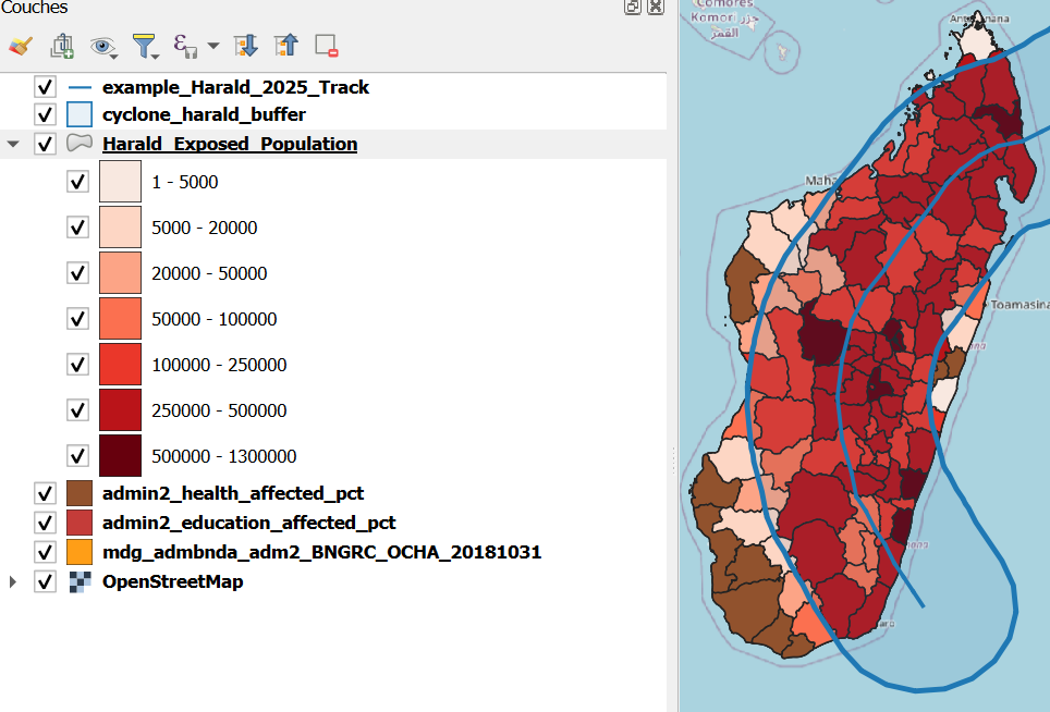
Carte montrant le nombre de personnes exposées par district après l’application du style .qml.

Intermediate result: Exposed Health Facilities

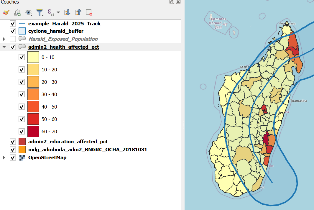
Carte indiquant le nombre total d’établissements de santé exposés par district, représentés avec le style prédéfini.

Intermediate result: Exposed Education Facilities

Carte affichant le nombre total d’établissements scolaires exposés par district, après application du fichier de style .qml.

3. Style Percentage Layers Manually

Aina also wants to visualise the percentage of exposed health and education facilities. However, since there is no prepared style available, she must complete the process manually.

Steps:

• Right-click on the layer admin2_health_affected → select Duplicate Layer

• Rename the duplicated layer to:

  admin2_health_affected_percentage
  

• Right-click on the layer in the Layers Panel

• Select Properties

• In the window that opens, go to the Symbology tab

• Set Symbology to Graduated

• Choose the correct field:

  • pct_health_affected

• Open the Histogram tab to view the value distribution by clicking on calculate histogram

• Next go back to Classes and set the following configuration:

  • Mode: Equal Interval

  • Classes: 4

• Click OK.This will create four classes (0–25%, 25–50%, 50–75%, 75–100%)

• Choose a color ramp (e.g., light yellow → dark red)

• Optionally customize class labels for clarity

• Click Apply

• Repeat the same process for the layer admin2_education_affected. After duplicating the layer, rename the new one to:

admin2_health_affected_percentage

🧠 Why 4 equal classes?
This helps visualize severity across districts using simple and interpretable risk categories. However, you can experiment with Natural Breaks if data is unevenly distributed.

---

4. Save Your New Styles for Reuse

Save your manually created styles as .qml files for future reuse.

Steps:

• Right-click on the layer in the Layers Panel

• Select Properties

• In the window that opens, go to the Symbology tab

• Click on Style → Save Style…

• Save the file in the folder layer_sytle

• Use these filenames:

  health_pct_affected_style
  

  education_pct_affected_style
  

5. (Optional) Import Styles into Your QGIS Library

To reuse your styles in any future project:

• Go to Settings → Style Manager

• Click Import/Export → Import Items

• Browse to and select your saved .qml files

The styles will now appear as presets in the Layer Styling Panel.

---

Task 5: Quick Map Creation – Aina Uses Map Templates

After all the hard work of analyzing data and styling layers, Aina is ready to share her results. But creating a professional-looking map from scratch every time would be slow and repetitive.

To save time, she uses map templates (.qpt files) prepared by her team. These templates already contain the essential elements — map frames, legends, logos, titles, and scale bars. With them, Aina can turn her analysis into a clean, consistent map in just a few clicks.

✅ Goal
Apply a ready-made QGIS map template to quickly create and export maps that show cyclone impacts on population, health facilities, and schools.

1. Load the pre-made print layout template

• Locate the template cyclone_impact_population_map_template.qpt in your project folder under:
  Map_Templates/

• You can load the template by drag-and-drop:

  • Open your QGIS project.

  • Drag the .qpt file directly into QGIS — a new layout will be created automatically.

• Alternatively:

  • Go to Project → New Print Layout

  • Enter a name (e.g. Harald_2025_population)

  • Click OK

  • In the layout, go to Layout → Import from Template…

  • Select the file cyclone_impact_overview_map_template.qpt and click Open

2. Check and set page size

• Right-click anywhere on the white canvas and choose Page Properties.

• On the right-side panel, ensure the following:

  • Page Size: A3

  • Orientation: Landscape

3. Update the attribute table of exposed districts

• In the Print Layout, click on the attribute table (right-hand side of the layout).

• In the Item Properties panel:

  • Ensure the correct layer is selected Harald_Exposed_population

  • Click Refresh Table Data

  • Click Attributes… → in the upper part under Fields click on Clear

    • Then add the following layer by clicking on ➕ :

    • Attribute: ADM1_EN; ADM2_EN; ADM2_PCODE; exposed_population_sum

    • To sort the tabel content, under the Sorting clicking on ➕ and add the column AMD1_EN

    • Sort Order: Ascending

  • Click OK

⚠️ Warning – Long Tables

If the attribute table you want to include is longer than the map frame, part of it will be cut off in the exported map.
To fix this, open the table properties in the layout and reduce the font size until the full table fits.

5. Adjust the legend

• In the layout, click on the Legend item.

• In the Item Properties panel:

  • Uncheck Auto update

  • Scroll to Legend items and remove all entries (🗑️)

  • Add the following relevant layers:

    • example_Harald_2025_Track

    • cyclone_harald_buffer

    • Harald_Exposed_Population

  • When selecting layers, check Only visible layers

  • Rename legend entries to match layout naming

    • example_Harald_2025_Track ->

    Cyclone Harald Track
    

    • cyclone_harald_buffer->

    Cyclone Harald 200 km Buffer
    

    • Harald_Exposed_Population->

    Number of exposed peopel
    

6. Update Logos and Icons

• The logos that need to be added to the map are represented by the red X.

• Click on the image in the Item List.

• Click on the three dots next to the file path.

• Browse to the folder logos_pictures and select the correct logo file.

7. Review and update layout text elements

• Make sure all text elements are up to date, especially:

  • Map title

  • Cyclone name and date

  • Author/Organization (optional)

• Adjust font size or alignment if necessary

✅ Final Checklist

Task	Done
Page set to A3 Landscape	☐
Only relevant layer group active	☐
Exposed districts attribute table updated	☐
Legend cleaned and renamed	☐
All text elements updated	☐

---

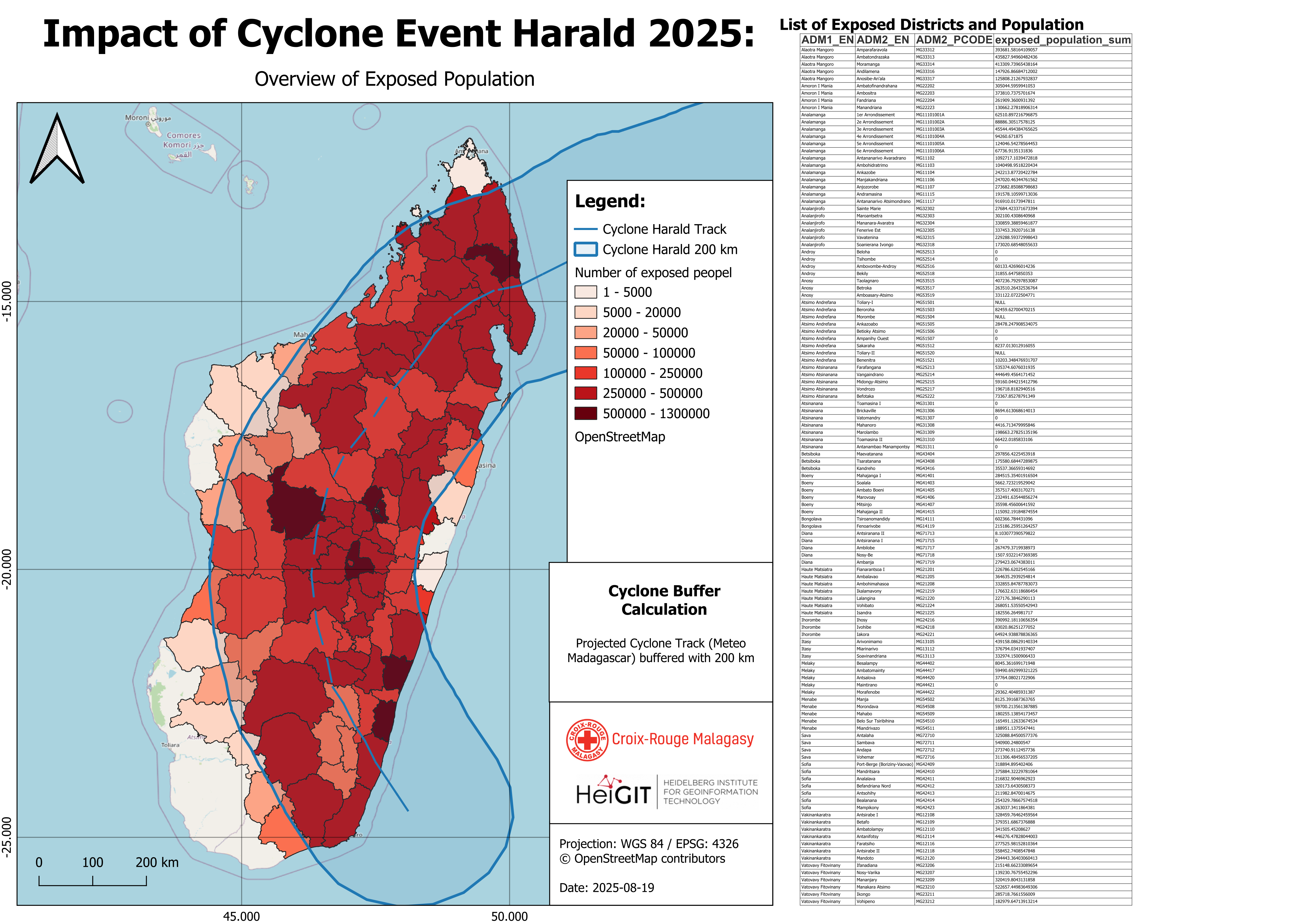
Your final output should look like this after styling the layer

The map now clearly displays the exposed population within the affected districts The original storm track line — used as input data — is highlighted, as well as the buffered impact area, which serves as a proxy for identifying exposed districts.

On the right-hand side of the map, a list shows all exposed districts, including data on total population and exposed population. The districts (Admin 2) are organized under their corresponding regions (Admin 1).

Task 6: Exporting Model Results for the Operations Team

Background – Aina Supports Decision Makers

After producing maps and visuals, Aina often gets requests from the operations team:

“Can you send us the data in table format?”

Instead of exporting these tables manually each time, Aina wants to automate this step within her model — ensuring that every run of the model produces clear, ready-to-use data files.

In this task, you’ll help Aina extend her existing model to export selected layers.

We will join the following layers step by step:

• admin2_health_affected_pct:
  Contains the total number of health facilities, the number of affected health facilities, and the percentage of affected health facilities.

• admin2_education_affected_pct:
  Contains the total number of education facilities, the number of affected education facilities, and the percentage of affected education facilities.

• exposed_population:
  Contains the total population per district and the exposed population from the zonal statistics step.

---

1. Open your model

• Open Estimate_Exposed_Population_Health_Education

• Save a new version as:

  Estimate_Exposed_Population_Health_Education_Spreadsheet_Export
  

2. Join Health and Education data into one layer

• In the Algorithms, search for Join Attributes by Field Value.

• Add a description: Joindre santé et éducation dans une seule couche par ADM2

• Configure the algorithm as follows:

  • Input Layer: admin2_health_affected (select from Algorithm Output)

  • Input Layer 2: admin2_education_affected (select from Algorithm Output)

  • Table field:

  ADM2_PCODE
  

  • Table field 2:

  ADM2_PCODE
  

  • Layer 2 fields to copy: Leave empty (all fields will be copied)

  • Join type: Take attributes of the first matching feature only (one-to-one)

  • Leave output as Model Output

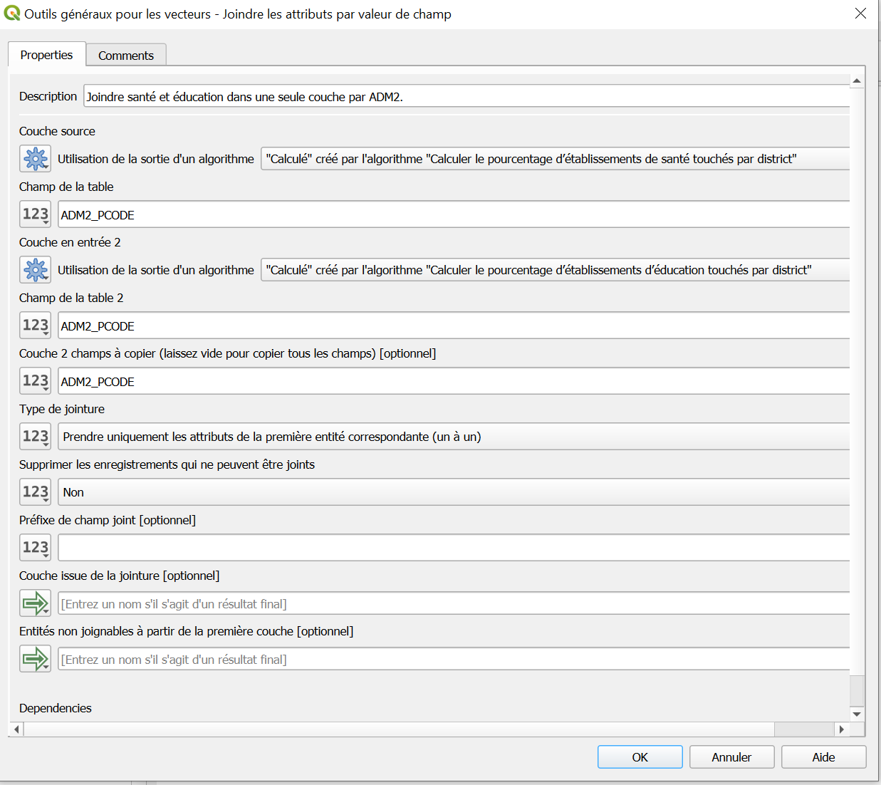
Configuration de l’opération : joindre les données de santé et d’éducation par le champ ADM2_PCODE afin de combiner les résultats dans une seule couche.

3. Join the result with the population data Now join the result of the previous step (health + education) to the exposed population data.

• Add a second Join Attributes by Field Value algorithm to the model

• Add a description: Joindre les données de population avec les indicateurs santé et éducation

• Configure the algorithm as follows:

  • Input Layer: exposed_population (select from Algorithm Output of the Zonal Statistics step)

  • Input Layer 2: Output from Step 2 (health + education)

  • Table field:

  ADM2_PCODE
  

  • Table field 2:

  ADM2_PCODE
  

  • Layer 2 fields to copy: (Enter the following field names exactly as shown — comma-separated, no spaces)

    count_health_total;sum_exposed_health;pct_exposed_health;count_education_total;sum_exposed_education;pct_exposed_education
    

  • Join type: Take attributes of the first matching feature only (one-to-one)

  • Leave output as Model Output

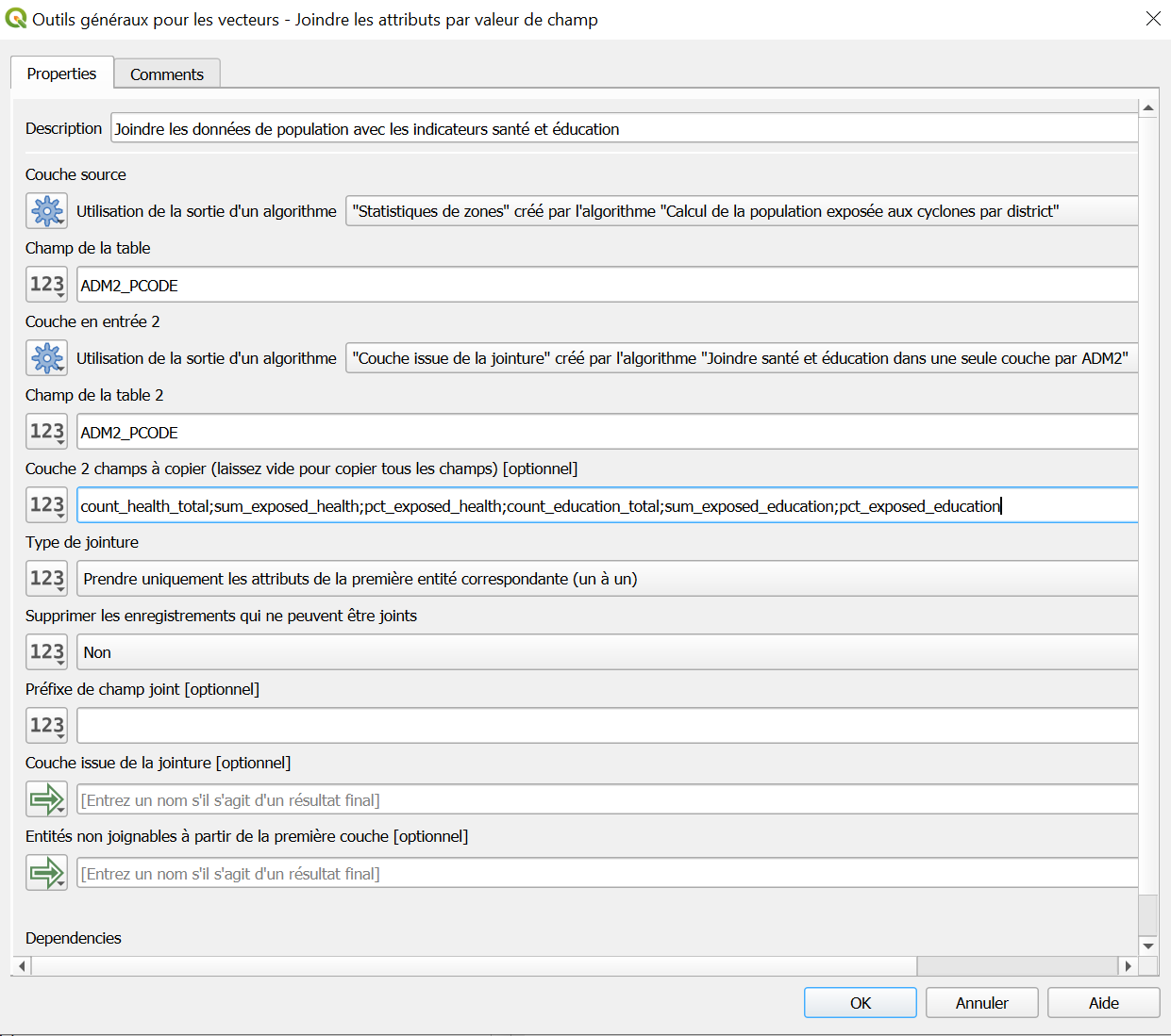
Configuration de l’opération : joindre les données de population avec les indicateurs de santé et d’éducation.

Tip

Where to find the column names
Open the attribute tables of the outputs health_total_per_admin2, sum_exposed_healthsites_POI, and admin2_health_affected_pct in QGIS.
Look at the column headers to find the exact names of the fields you want to copy.

Warning

Invisible spaces will break the join
If a column name like count_health_total has an invisible trailing space, the join will silently fail.
Always copy field names directly from the attribute table to avoid errors.

4. Export results to a spreadsheet

• In the Processing Toolbox, search for Export to spreadsheet and double-click to open.

• Add a description: Exporter les données de population, d'éducation et de santé dans un seul tableau

• Configure the tool as follows:

  • Input Layer: Select the output of Step 3 from Algorithm Output

  • Destination spreadsheet:

    exposure_indicators_spreadsheet
    

  • Click OK to add it to the model. Once you run the model, this step will automatically generate a spreadsheet with all relevant indicators ready for the operations team!

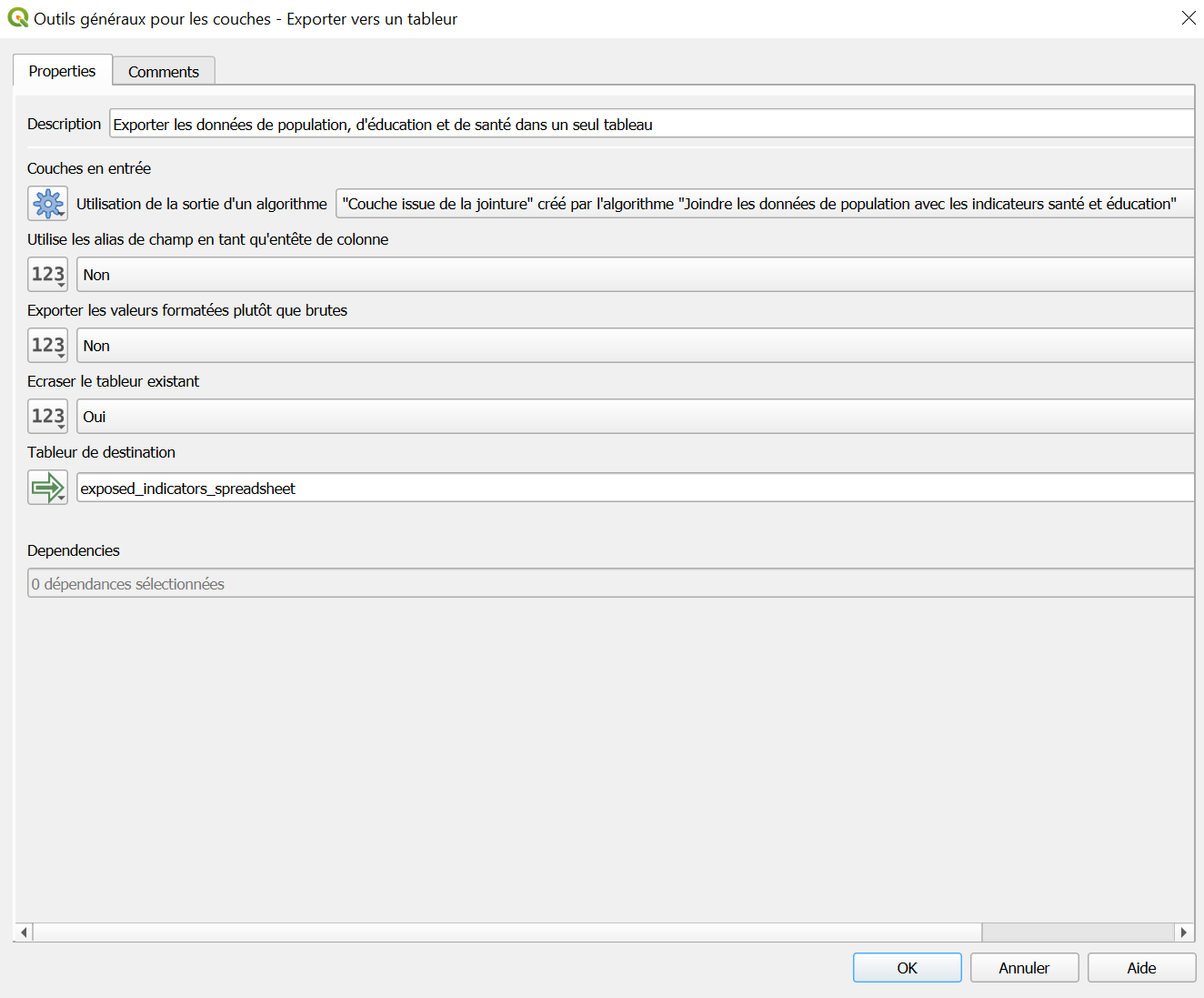
Exporter tous les indicateurs (population, santé, éducation) vers un tableau unique au format tableur.

5. Validate and Save Your Extended Model

   • Click the ✔️ Validate Model button to check for errors.

   • Save again to:
     Estimate_Exposed_Population_Health_Education.model3

6. Run the model

   • Click the ▶️ Run button in the top-right corner of the Graphical Modeler window.

   • Input:

     • Click on the three dots for each input dataset and select the correct input:

       • Cyclone Track → select the GeoJSON of the storm path (e.g. Harald_2025_Track.geojson)

       • Population Raster → select the WorldPop raster file

       • Admin Boundaries → select the Admin 2 layer (e.g. MDG_adm2.gpkg)

       • Health Facilities → select the point dataset for health sites

       • Education Facilities → select the point dataset for schools

   • Output:

     • Save all output layers in the output folder and use the names below.

       • admin2_health_affacted ->

       admin2_health_affected
       

       • admin2_education_affected ->

       admin2_education_affected
       

       • cyclone_harald_buffer ->

       cyclone_harald_buffer
       

       • exposed_population_sum ->

       admin2_harald_Exposed_Population
       

       • exposure_indicators_spreadsheet ->

       exposure_indicators_harald
       

   • Click Run to execute the full model.

Graphic Modler

Vue du modeleur graphique avec l’étape d’exportation vers un tableau ajoutée au modèle.

Run Model Configuration

Fenêtre de configuration pour exécuter le modèle avec l’option d’export vers un tableau.

Model Output

Résultats finaux du modèle exportés dans un tableau prêt à être utilisé.

---

Task 7: Reachability of health Posts from CRM Warehouses

Context:

When a cyclone is forecast to make landfall, Aina works with the logistics and health teams to decide where to send prepositioned medical kits. However, not all CRM warehouses stock the needed items — only three do.

To make fast, data-driven decisions, Aina wants to know which health posts are reachable from those warehouses within 10 hours. This analysis helps ensure that kits are sent to facilities that can actually be reached in time.

Her goal is to create a clear visual map showing reachable vs. non-reachable health posts — and share this with decision-makers as quickly as possible.

1. Filter Health Posts from the National Health Facility Dataset

Before checking which facilities are reachable, Aina needs to isolate health posts from the broader dataset of all health facilities.

1. Load the health facilities dataset

   • File: hotosm_mdg_health_facilities_points.gpkg (or the respective GeoPackage you are using)

   • Load it via drag and drop or through Layer → Add Vector Layer.

2. Open the attribute table and check the column named amenity.

3. Filter by expression to keep only health posts:

   • Right-click the layer → Filter…

   • Use the following expression:

     "amenity" = 'health_post'
     

4. Export the filtered layer

   • Right-click the filtered layer in the Layers Panel → Export → Save Features As…

   • Format: GeoPackage

   • Save to your project folder as:

     health_posts_only.gpkg
     

   • Click OK to confirm export.

5. Remove the filter or original layer from your project to avoid confusion.

💡 Tip: Filtering directly in QGIS lets you work with a specific subset of features without modifying the original dataset.

2. Load Isochrone Layers for the Three CRM Warehouses

Aina knows that only three warehouses stock the necessary medical supplies:
Antananarivo, Maroantsetra, and Tolanaro. She will now load the isochrone layers for each of these warehouses to begin analyzing service areas.

1. Load the individual isochrone layers for each warehouse:

   • CRM_warehouse_Isochrones_Antananarivo.gpkg

   • CRM_warehouse_Isochrones_Maroantsetra.gpkg

   • CRM_warehouse_Isochrones_Tolanaro.gpkg

   You can drag and drop each file into QGIS or go to Layer → Add Layer → Add Vector Layer.

2. Inspect the attribute table of each isochrone layer
   Confirm that each record has a traveltime_h field showing the estimated travel time in hours.

3. Remove all features where travel time is above 10 hours:

   • Right-click each layer → Filter…

   • Apply the expression:

     "traveltime_h" <= 10
     

4. Export each filtered layer to the temp folder : At this point, Aina also ensures all exported layers are saved in the same CRS as the health post dataset — EPSG:4326 — to avoid problems in the spatial join.

   • Save each as:

     CRM_isochrones_Antananarivo_upto10h.gpkg
     CRM_isochrones_Maroantsetra_upto10h.gpkg
     CRM_isochrones_Tolanaro_upto10h.gpkg
     

5. Style the isochrones for clarity Aina can apply predefined style file to color the layer based on traveltime_h to visualize different time bands (4h, 6h, 8h, 10h) later in Step 5.

   • Right-click each filtered layer → Properties → Symbology

   • Click Style at the bottom → Load Style…

   • Select the file:
     CRM_warehouse_isochrones_style.qml

   • Click Open, then Apply and OK

3. Visualizing Health Post Reachability from CRM Warehouses

Aina needs to identify which health posts can be reached by road from three key CRM warehouses (Antananarivo, Maroantsetra, and Tolanaro) within 10 hours of travel time. She will do this manually by combining the 10-hour isochrones from these warehouses and comparing them to the national health post dataset.

1. Merge the Isochrone Layers from the Three Warehouses

   • In the Processing Toolbox, search for Merge Vector Layers.

   • Input layers:

     • CRM_isochrones_Antananarivo_upto10h.gpkg

     • CRM_isochrones_Maroantsetra_upto10h.gpkg

     • CRM_isochrones_Tolanaro_upto10h.gpkg

   • CRS: EPSG:4326

   • Save to file:

     merged_isochrones_10h.gpkg
     

   • Click Run.

2. Select Health Posts Reachable Within 10 Hours

   • In the Processing Toolbox, search for Select by Location.

   • Set the following parameters:

     • Input layer: health_posts_only.gpkg

     • Predicate: intersects

     • Intersect layer: merged_isochrones_10h.gpkg

   • Click Run.

   💡 The selected points are those within the 10-hour service areas of the warehouses.

3. Create a Reachability Field for Selected Health Posts

   • Open the Field Calculator on the health_posts_only layer.

   • Check ✅ Only update selected features

   • Output field name: Reachability_time

   • Output field type: Text (string)

   • Expression:

     'reachable in 10 hours'
     

   • Click OK to create and populate the new field for selected features.

4. Mark the Remaining Health Posts as Not Reachable

   • Invert the selection:
     Go to Edit → Invert Feature Selection
     or right-click the layer and select Invert Selection.

   • Open the Field Calculator again.

   • Check ✅ Only update selected features

   • Use the same field: Reachability_time

   • Expression:

     'not reachable in 10 hours'
     

   • Click OK to apply the update.

✅ Now all health posts are labeled as either reachable or not reachable in the Reachability_time column.