Query openrouteservice from R

Get started

openrouteservice R package provides easy access to the openrouteservice (ORS) API from R. It allows you to painlessly consume the following services:

directions (routing)
geocode powered by Pelias
isochrones (accessibility)
time-distance matrix
pois (points of interest)
SRTM elevation for point and lines geometries
routing optimization based on Vroom

Disclaimer

By using this package, you agree to the ORS terms and conditions.

Installation

The package is not yet available from CRAN, but you can install the development version directly from GitHub.

# install.packages("remotes")
remotes::install_github("GIScience/openrouteservice-r")

Setting up API key

In order to start using ORS services you first need to set up your personal API key, which you can get for free. Once you are signed up, go to https://openrouteservice.org/dev/#/home -> TOKENS. At the bottom of the page you can request a free token (name can be anything).

library(openrouteservice)

ors_api_key("<your-api-key>")

This will save the key in the default keyring of your system credential store. Once the key is defined, it persists in the keyring store of the operating system. This means that it survives beyond the termination of the R session, so you don’t need to set it again each time you start a new R session. To retrieve the key just call ors_api_key() without the key argument.

Alternatively, they key can be provided in the environment variable ORS_API_KEY. The value from the environment variable takes precedence over the former approach allowing to bypass the keyring infrastructure.

Directions

ors_directions() interfaces the ORS directions service to compute routes between given coordinates.

library(openrouteservice)

coordinates <- list(c(8.34234, 48.23424), c(8.34423, 48.26424))

x <- ors_directions(coordinates)

Way points can be provided as a list of coordinate pairs c(lon, lat), or a 2-column matrix-like object such as a data frame.

coordinates <- data.frame(lon = c(8.34234, 8.34423), lat = c(48.23424, 48.26424))

The response formatting defaults to geoJSON which allows to easily visualize it with e.g. leaflet.

library(leaflet)

leaflet() %>%
  addTiles() %>%
  addGeoJSON(x, fill=FALSE) %>%
  fitBBox(x$bbox)

Other output formats, such as GPX, can be specified in the argument format. Note that plain JSON response returns the geometry as Google’s encoded polyline,

x <- ors_directions(coordinates, format = "json")

geometry <- x$routes[[1]]$geometry
str(geometry)

##  chr "mtkeHuv|q@~@VhAf@PR|@hBt@j@^n@L\\NjAX`BNXqAlFM^kArAoAfBs@^WFY?{Be@[?WJWRi@t@Q^]`AQRULoAPWHOL]h@mA`C_@d@oAdAkCrB"| __truncated__

so an additional postprocessing step might be necessary.

library(googlePolylines)
str(decode(geometry))

## List of 1
##  $ :'data.frame':    166 obs. of  2 variables:
##   ..$ lat: num [1:166] 48.2 48.2 48.2 48.2 48.2 ...
##   ..$ lon: num [1:166] 8.34 8.34 8.34 8.34 8.34 ...

The API offers a wide range of profiles for multiple modes of transport, such as: car, heavy vehicle, different bicycle types, walking, hiking and wheelchair. These can be listed with

ors_profile()

##                car                hgv               bike           roadbike                mtb 
##      "driving-car"      "driving-hgv"  "cycling-regular"     "cycling-road" "cycling-mountain" 
##             e-bike            walking             hiking         wheelchair 
## "cycling-electric"     "foot-walking"      "foot-hiking"       "wheelchair"

Each of these modes uses a carefully compiled street network to suite the profiles requirements.

x <- ors_directions(coordinates, profile="cycling-mountain")

leaflet() %>%
  addTiles() %>%
  addGeoJSON(x, fill=FALSE) %>%
  fitBBox(x$bbox)

Any optional query parameters can be specified by providing them as additional ... arguments to ors_directions. For example, in order to plot the elevation profile of a route colored by steepness use elevation = TRUE to add height to the coordinates of the points along the route and query for steepness in extra_info.

library("sf")

x <- ors_directions(coordinates, profile = "cycling-mountain", elevation = TRUE,
                    extra_info = "steepness", output = "sf")

height <- st_geometry(x)[[1]][, 3]

Here we use simple features output for the sake of easy postprocessing which includes finding the length of individual route segments and their distance relative to the starting point. These can be computed with st_distance() upon converting the LINESTRING to a list of POINTs,

points <- st_cast(st_geometry(x), "POINT")
n <- length(points)
segments <- cumsum(st_distance(points[-n], points[-1], by_element = TRUE))

## st_as_s2(): dropping Z and/or M coordinate
## st_as_s2(): dropping Z and/or M coordinate

while their steepness can be extracted from the requested metadata.

steepness <- x$extras$steepness$values
steepness <- rep(steepness[,3], steepness[,2]-steepness[,1])
steepness <- factor(steepness, -5:5)

palette = setNames(rev(RColorBrewer::brewer.pal(11, "RdYlBu")), levels(steepness))

For the final plot we use ggplot2 in combinations with ggforce which supports handling of length units associated with the data.

library("ggplot2")
library("ggforce")
library("units")

units(height) <- as_units("m")

df <- data.frame(x1 = c(set_units(0, "m"), segments[-(n-1)]),
                 x2 = segments,
                 y1 = height[-n],
                 y2 = height[-1],
                 steepness)

y_ran = range(height) * c(0.9, 1.1)

n = n-1

df2 = data.frame(x = c(df$x1, df$x2, df$x2, df$x1),
                 y = c(rep(y_ran[1], 2*n), df$y2, df$y1),
                 steepness,
                 id = 1:n)

ggplot() + theme_bw() +
  geom_segment(data = df, aes(x1, y1, xend = x2, yend = y2), size = 1) +
  geom_polygon(data = df2, aes(x, y, group = id), fill = "white") +
  geom_polygon(data = df2, aes(x, y , group = id, fill = steepness)) +
  scale_fill_manual(values = alpha(palette, 0.8), drop = FALSE) +
  scale_x_unit(unit = "km", expand = c(0,0)) +
  scale_y_unit(expand = c(0,0), limits = y_ran) +
  labs(x = "Distance", y = "Height")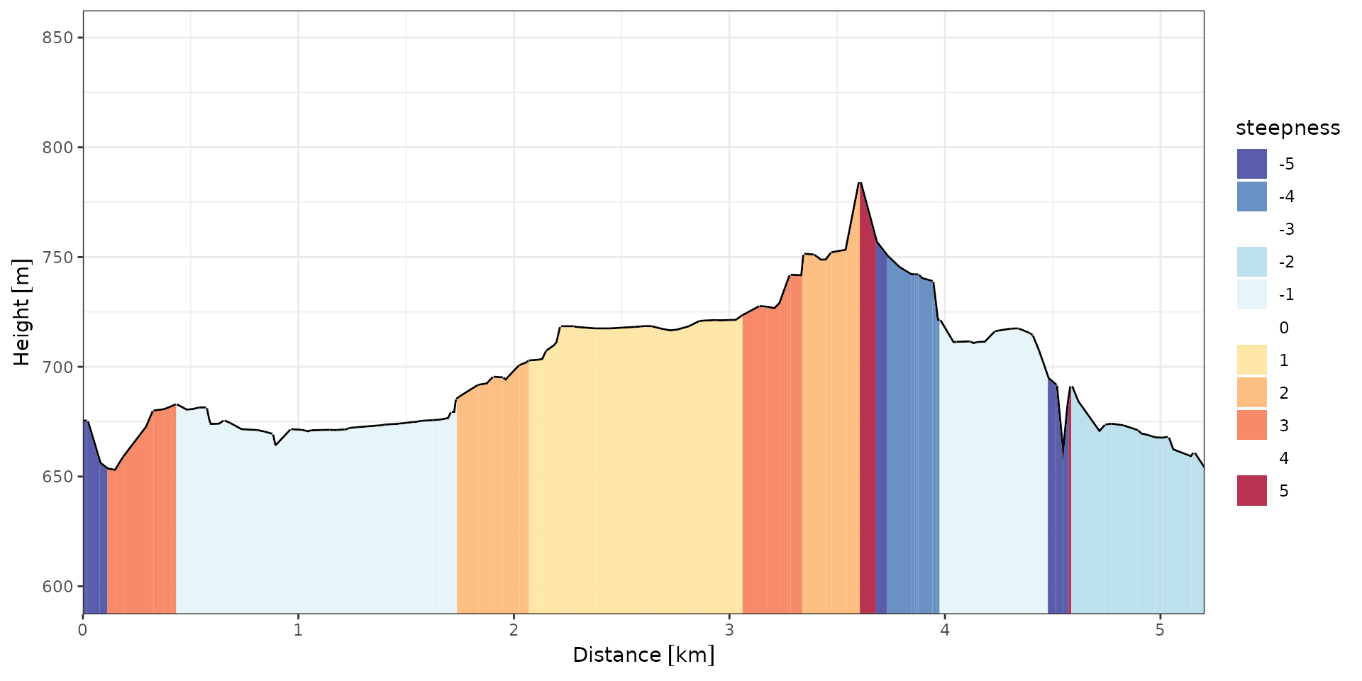

## Warning: Using `size` aesthetic for lines was deprecated in ggplot2 3.4.0.
## ℹ Please use `linewidth` instead.
## This warning is displayed once every 8 hours.
## Call `lifecycle::last_lifecycle_warnings()` to see where this warning was generated.

## Warning: `scale_x_unit()` was deprecated in ggforce 0.3.4.
## ℹ Please use `units::scale_x_unit()` instead.
## This warning is displayed once every 8 hours.
## Call `lifecycle::last_lifecycle_warnings()` to see where this warning was generated.

## Warning: `scale_y_unit()` was deprecated in ggforce 0.3.4.
## ℹ Please use `units::scale_y_unit()` instead.
## This warning is displayed once every 8 hours.
## Call `lifecycle::last_lifecycle_warnings()` to see where this warning was generated.

Advanced options are natively formatted as JSON objects, but can be passed as their R list representation.

polygon = list(
    type = "Polygon",
    coordinates = list(
      list(
        c(8.330469, 48.261570),
        c(8.339052, 48.261570),
        c(8.339052, 48.258227),
        c(8.330469, 48.258227),
        c(8.330469, 48.261570)
      )
    ),
    properties = ""
  )

options <- list(
  avoid_polygons = polygon
)

x <- ors_directions(coordinates, profile="cycling-mountain", options=options)

leaflet() %>%
  addTiles() %>%
  addGeoJSON(polygon, color="#F00") %>%
  addGeoJSON(x, fill=FALSE) %>%
  fitBBox(x$bbox)

Isochrones

Reachability has become a crucial component for many businesses from all different kinds of domains. ors_isochrones() helps you to determine which areas can be reached from certain location(s) in a given time or travel distance. The reachability areas are returned as contours of polygons. Next to the range provided in seconds or meters you may as well specify the corresponding intervals. The list of optional arguments to ors_isochrones() is similar as to ors_directions().

library(mapview)

## The legacy packages maptools, rgdal, and rgeos, underpinning the sp package,
## which was just loaded, will retire in October 2023.
## Please refer to R-spatial evolution reports for details, especially
## https://r-spatial.org/r/2023/05/15/evolution4.html.
## It may be desirable to make the sf package available;
## package maintainers should consider adding sf to Suggests:.
## The sp package is now running under evolution status 2
##      (status 2 uses the sf package in place of rgdal)

# embed data in the output file
mapviewOptions(fgb = FALSE)

coordinates <- data.frame(lon = c(8.34234, 8.34234), lat = c(48.23424, 49.23424))

## 30 minutes range split into 10 minute intervals
res <- ors_isochrones(coordinates, range = 1800, interval = 600, output = "sf")
res

## Simple feature collection with 6 features and 3 fields
## Geometry type: POLYGON
## Dimension:     XY
## Bounding box:  xmin: 8.043995 ymin: 48.08958 xmax: 8.691726 ymax: 49.51392
## Geodetic CRS:  WGS 84
##   group_index              center value                       geometry
## 1           0 8.344268, 48.233826   600 POLYGON ((8.259945 48.22342...
## 2           0 8.344268, 48.233826  1200 POLYGON ((8.201708 48.23176...
## 3           0 8.344268, 48.233826  1800 POLYGON ((8.103483 48.19896...
## 4           1 8.343705, 49.234211   600 POLYGON ((8.278396 49.24286...
## 5           1 8.343705, 49.234211  1200 POLYGON ((8.147534 49.26519...
## 6           1 8.343705, 49.234211  1800 POLYGON ((8.043995 49.27217...

values <- levels(factor(res$value))
ranges <- split(res, values)
ranges <- ranges[rev(values)]

names(ranges) <- sprintf("%s min", as.numeric(names(ranges))/60)

mapview(ranges, alpha.regions = 0.2, homebutton = FALSE, legend = FALSE)

Here we have used sf output for the sake of some further postprocessing and visualization. By grouping the isochrones according to ranges we gain the ability of toggling individual ranges when displayed in mapview. Another option could be to group by locations. The following example illustrates a possible approach to applying a custom color palette to the non-overlapping parts of isochrones.

locations = split(res, res$group_index)

locations <- lapply(locations, function(loc) {
  g <- st_geometry(loc)
  g[-which.min(values)] <- st_sfc(Map(st_difference,
                                      g[match(values[-which.min(values)], loc$value)],
                                      g[match(values[-which.max(values)], loc$value)]))
  st_geometry(loc) <- g
  loc
})

isochrones <- unsplit(locations, res$group_index)

pal <- setNames(heat.colors(length(values)), values)
mapview(isochrones, zcol = "value", col = pal, col.regions = pal,
        alpha.regions = 0.5, homebutton = FALSE)

Matrix

One to many, many to many or many to one: ors_matrix() allows you to obtain aggregated time and distance information between a set of locations (origins and destinations). Unlike ors_directions() it does not return detailed route information. But you may still specify the transportation mode and compute routes which adhere to certain restrictions, such as avoiding specific road types or object characteristics.

coordinates <- list(
  c(9.970093, 48.477473),
  c(9.207916, 49.153868),
  c(37.573242, 55.801281),
  c(115.663757,38.106467)
)

# query for duration and distance in km
res <- ors_matrix(coordinates, metrics = c("duration", "distance"), units = "km")

# duration in hours
(res$durations / 3600) %>% round(1)

##       [,1]  [,2] [,3]  [,4]
## [1,]   0.0   1.6 25.2 109.7
## [2,]   1.6   0.0 25.1 109.5
## [3,]  25.1  25.0  0.0  85.6
## [4,] 109.5 109.3 85.3   0.0

# distance in km
res$distances %>% round

##      [,1] [,2] [,3] [,4]
## [1,]    0  154 2411 9860
## [2,]  154    0 2385 9835
## [3,] 2359 2334    0 7501
## [4,] 9791 9767 7449    0

Geocoding

ors_geocode() transforms a description of a location provided in query, such as the place’s name, street address or postal code, into a normalized description of the location with a point geometry. Additionally, it offers reverse geocoding which does exactly the opposite: It returns the next enclosing object which surrounds the coordinates of the given location. To obtain more relevant results you may also set a radius of tolerance around the requested coordinates.

## locations of Heidelberg around the globe
x <- ors_geocode("Heidelberg")

leaflet() %>%
  addTiles() %>%
  addGeoJSON(x) %>%
  fitBBox(x$bbox)

## set the number of results returned
x <- ors_geocode("Heidelberg", size = 1)

## search within a particular country
x <- ors_geocode("Heidelberg", boundary.country = "DE")

## structured geocoding
x <- ors_geocode(list(locality="Heidelberg", county="Heidelberg"))

## reverse geocoding
location <- x$features[[1L]]$geometry$coordinates

y <- ors_geocode(location = location, layers = "locality", size = 1)

POIs

This service allows you to find places of interest around or within given geographic coordinates. You may search for given features around a point, path or even within a polygon specified in geometry. To list all the available POI categories use ors_pois('list').

geometry <- list(
  geojson = list(
    type = "Point",
    coordinates = c(8.8034, 53.0756)
  ),
  buffer = 500
)

ors_pois(
  request = 'pois',
  geometry = geometry,
  limit = 2000,
  sortby = "distance",
  filters = list(
    category_ids = 488,
    wheelchair = "yes"
  ),
  output = "sf"
)

## Simple feature collection with 3 features and 5 fields
## Geometry type: POINT
## Dimension:     XY
## Bounding box:  xmin: 8.80294 ymin: 53.07452 xmax: 8.80903 ymax: 53.0757
## Geodetic CRS:  WGS 84
##       osm_id osm_type  distance category_ids osm_tags                 geometry
## 1  726580652        1  32.95127 kiosk, shops      yes  POINT (8.80294 53.0757)
## 2 2525463951        1 292.89365 kiosk, shops      yes POINT (8.80777 53.07559)
## 3 4827632819        1 395.87884 kiosk, shops      yes POINT (8.80903 53.07452)

You can gather statistics on the amount of certain POIs in an area by using request='stats'.

ors_pois(
  request = 'stats',
  geometry = geometry,
  limit = 2000,
  sortby = "distance",
  filters = list(category_ids = 488)
  )

## <ors_pois>
## List of 2
##  $ places     :List of 2
##   ..$ total_count: int 8
##   ..$ shops      :List of 3
##   .. ..$ group_id   : int 420
##   .. ..$ categories :List of 1
##   .. .. ..$ kiosk:List of 2
##   .. .. .. ..$ count      : int 8
##   .. .. .. ..$ category_id: int 488
##   .. ..$ total_count: int 8
##  $ information:List of 4
##   ..$ attribution: chr "openrouteservice.org | OpenStreetMap contributors"
##   ..$ version    : chr "0.1"
##   ..$ timestamp  : int 1695215020
##   ..$ query      :List of 5
##   .. ..$ request : chr "stats"
##   .. ..$ limit   : int 2000
##   .. ..$ sortby  : chr "distance"
##   .. ..$ filters :List of 1
##   .. .. ..$ category_ids: int 488
##   .. ..$ geometry:List of 2
##   .. .. ..$ geojson:List of 2
##   .. .. .. ..$ type       : chr "Point"
##   .. .. .. ..$ coordinates: num [1:2] 8.8 53.1
##   .. .. ..$ buffer : int 500

Elevation

Given a point or line geometry you can use ors_elevation to query for its elevation.

x <- ors_geocode("Königstuhl", output = "sf")

ors_elevation("point", st_coordinates(x))

## <ors_elevation>
##  num [1:3] 8.72 49.4 560

Optimization

The optimization endpoint solves the vehicle routing problem (VRP) of finding an optimal set of routes for a fleet of vehicles to traverse in order to deliver to a given set of locations. The service is based on Vroom and can be used to schedule multiple vehicles and jobs respecting time windows, capacities and required skills. VRP generalizes the classic traveling salesman problem of finding the fastest or shortest possible route that visits a given list of locations.

The following example involves a 2-vehicle fleet carrying out deliveries across 6 locations.

home_base <- data.frame(lon = 2.370658, lat = 48.721666)

vehicles = vehicles(
  id = 1:2,
  profile = "driving-car",
  start = home_base,
  end = home_base,
  capacity = 4,
  skills = list(c(1, 14), c(2, 14)),
  time_window = c(28800, 43200)
)

Both vehicles share the start/end points and have the same capacity, but differ in the set of skills assigned. We are interested in using them to serve a number of jobs with certain skills requirements between locations. These skills are mandatory, which means a given job can only be served by a vehicle that has all its required skills.

locations <- list(
  c(1.98806, 48.705),
  c(2.03655, 48.61128),
  c(2.39719, 49.07611),
  c(2.41808, 49.22619),
  c(2.28325, 48.5958),
  c(2.89357, 48.90736)
)

jobs = jobs(
  id = 1:6,
  service = 300,
  amount = 1,
  location = locations,
  skills = list(1, 1, 2, 2, 14, 14)
)

The helper functions vehicles and jobs produce data.frames which have the format appropriate for ors_optimization. Route geometries are enabled by setting the corresponding flag in options.

res <- ors_optimization(jobs, vehicles, options = list(g = TRUE))

The geometries are returned as Google’s encoded polylines, so for visualization in leaflet they need to be decoded. Furthermore, we extract the job locations from the response such that we can label them in the order in which they are visited along the routes.

lapply(res$routes, with, {
  list(
    geometry = googlePolylines::decode(geometry)[[1L]],
    locations = lapply(steps, with, if (type=="job") location) %>%
      do.call(rbind, .) %>% data.frame %>% setNames(c("lon", "lat"))
  )
  }) -> routes

## Helper function to add a list of routes and their ordered waypoints
addRoutes <- function(map, routes, colors) {
  routes <- mapply(c, routes, color = colors, SIMPLIFY = FALSE)
  f <- function (map, route) {
    with(route, {
      labels <- sprintf("<b>%s</b>", 1:nrow(locations))
      markers <- awesomeIcons(markerColor = color, text = labels, fontFamily = "arial")
      map %>%
        addPolylines(data = geometry, lng = ~lon, lat = ~lat, col = ~color) %>%
        addAwesomeMarkers(data = locations, lng = ~lon, lat = ~lat, icon = markers)
    })
  }
  Reduce(f, routes, map)
}

leaflet() %>%
  addTiles() %>%
  addAwesomeMarkers(data = home_base, icon = awesomeIcons("home")) %>%
  addRoutes(routes, c("purple", "green"))

Andrzej Oleś

2023-09-20