7 Calculate redundancy
7.1 Research Question 3
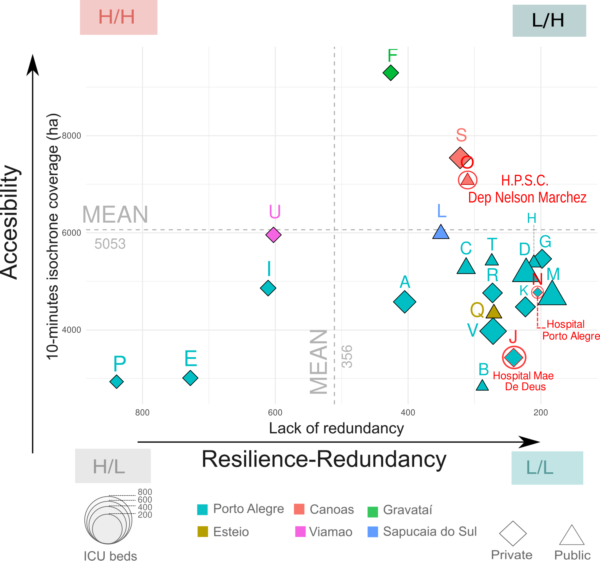
Which healthcare facility was the least resilient in terms of redundancy?
Figure 7.1 includes the healthcare facilities of the Core Metropolitan Area their bed capacity, their accessibility and lack of resilience in terms of redundancy. The size of each point is related to the number of beds, while the shape represent if it is a public or private entity. We measured the accesibility on the y-axis by the surface covered in 10 minutes by car from each healthcare facilities The x-axis represents the lack of redundancy based on the difference on alternatives routes to the healthcare facilities coloured in red intersected with the flood extent.
High lack of redundancy highlights cases like Hospital Restinga e Extremo Sul, where the alternative paths vary greatly in distance. This suggests poor resilience, where disruptions from the flood result in inefficient and costly. On the contrary, low lack of redundancy values indicates similar distances in the alternative routes to the hospital showing a higher resilience. The most resilient hospitals in terms of lack of redundancy are those located in the quadrant “L/H” with a low lack of redundancy and high accesibility in terms of coverage.
How to create the base for Figure 7.1.
## Import data, if it is not already
isochrone_ghs_aoi <- sf::read_sf("~/agile-gscience-2024-rs-flood/data/rmarkdown_data/isochrone_ghs_aoi.gpkg")
resilience_visintini_table <- sf::read_sf("~/agile-gscience-2024-rs-flood/data/rmarkdown_data/resilience_visintini_table.gpkg")
## Data wrangling
plot_resilience_v2 <-  resilience_visintini_table |>
  mutate(rank = rank(resilience_visintini_table$lack_pre),
         municipality = resilience_visintini_table$shapename,
         letter = LETTERS[1:length(resilience_visintini_table$ds_cnes)],
         area_hm_2 = round(st_area(isochrone_ghs_aoi)),
          lack_norm = (lack_pre - min(lack_pre)) / (max(lack_pre) - min(lack_pre)),
         ds_cnes=stringr::str_to_title(ds_cnes)) |>
  sf::st_drop_geometry() |>
  select(c(rank,letter,ds_cnes, municipality, lack_pre,beds, lack_post,lack_norm, beds, code, area_hm_2)) |>
  arrange(lack_pre)
## Transform by adding area in hm² and adding mean for both axis.
plot_resilience_v2$area_hm_2 <-  units::set_units(plot_resilience_v2$area_hm_2, "hm^2")
x_mid <- mean(c(max(plot_resilience_v2$lack_pre, na.rm = TRUE), min(plot_resilience_v2$lack_pre, na.rm = TRUE)))
y_mid <- mean(c(max(plot_resilience_v2$area_hm_2, na.rm = TRUE), min(plot_resilience_v2$area_hm_2, na.rm = TRUE)))

## Visualize data
ggplot(plot_resilience_v2, aes(x = lack_pre, y = area_hm_2, shape=code, colour=municipality)) +
    geom_vline(xintercept = x_mid, linetype="dashed", linewidth=0.5, colour="darkgray") +
    geom_hline(yintercept = y_mid, linetype="dashed", linewidth=0.5, colour="darkgray") +
    ggplot2::geom_text(aes(label=letter), vjust=-1.5, size=5, show.legend = FALSE) +
    geom_point(aes(shape = code, colour = municipality, fill=municipality, size = beds)) +
   scale_size(range = c(3.5,10)) +
  scale_shape_manual(values = c(23, 24))  +
  expand_limits(y= units::set_units(c(2800, 9500),"hm^2"), x=c(150,850)) +
  scale_x_reverse() +
  annotate("text",
           x = filter(plot_resilience_v2, lack_post ==0)$lack_pre[1],
           y = filter(plot_resilience_v2, lack_post ==0)$area_hm_2[1],
           label=filter(plot_resilience_v2, lack_post ==0)$ds_cnes[1],
           colour="red") +
  annotate("text",
           x = filter(plot_resilience_v2, lack_post ==0)$lack_pre[2],
           y = filter(plot_resilience_v2, lack_post ==0)$area_hm_2[2],
           label=filter(plot_resilience_v2, lack_post ==0)$ds_cnes[2],
           colour="red") +
    annotate("text",
           x = filter(plot_resilience_v2, lack_post ==0)$lack_pre[3],
           y = filter(plot_resilience_v2, lack_post ==0)$area_hm_2[3],
           label=filter(plot_resilience_v2, lack_post ==0)$ds_cnes[3],
           colour="red") +
  xlab("Lack of redundancy") +
  ylab("10-minutes isochrone coverage") +
  theme_minimal() +
  theme(legend.position = "bottom")

## Manual fine adjustments done with the open-source software Inkscape
The data is contained in the Table 7.1
7.1.1 Alternative route function
The code ACR-1 created three least-cost paths with a penalty methods in each iteration asssssing the lack of redundancy of the healthcare facilities’ access. The variable hospital_name at the line 4 used the name of the healthcare facilities as the destination of the least-cost paths, while the variable origin_id was the origin regularly sampled within the healthcare facilities. The lines located from 15 to 203 iterated for each point related to each healthcare facilities. The penalty method is applied in the line 57 and 114 increasing the costs of the previous least-cost paths finding alternative routes.
[ACR-1] How to create a function to calculate alternative paths with a penalty method
alternative_routes <- function(df_isochrone_points){
  for (idx in 1:length(df_isochrone_points$id)) {
    tic(glue("run {idx}/{length(df_isochrone_points$id)}"))
    hospital_name <- df_isochrone_points$cd_cnes[idx]
    origin_id <- df_isochrone_points$id[idx]

    table_name_1 <- glue("first_path_point_{as.character(idx)}")
    table_name_2 <- glue("second_path_point_{as.character(idx)}")
    table_name_3 <- glue("second_route_point_{as.character(idx)}")
    table_name_4 <- glue("third_path_point_{as.character(idx)}")
    table_name_5 <- glue("third_route_point_{as.character(idx)}")
    table_name_6 <- glue("three_alternative_routes_point_{as.character(idx)}")
    table_name_7 <- glue("table_end_point_{as.character(idx)}")

#### First shortest path
dbExecute(glue_sql("DROP TABLE IF EXISTS {`table_name_1`}", .con=connection),
          conn=connection)
query_1 <- glue_sql("
CREATE TABLE {`table_name_1`} AS
SELECT
        seq,
        path.start_vid,
        path.end_vid,
        path.node,
        path.edge,
        net.the_geom,
        path.cost,
        path.agg_cost,
        1 AS path
  FROM pgr_dijkstra('
        SELECT
            id,
            source,
            target,
            cost
        FROM ghs_aoi_net_largest_renamed',
                    ARRAY(SELECT id FROM regular_sampling_isochrones_snapped_ghs_aoi WHERE id ={origin_id}),
                    ARRAY(SELECT id AS end_id FROM municipalities_ghs_hospitals WHERE cd_cnes = {hospital_name}),
                    directed:=TRUE) AS path
LEFT JOIN ghs_aoi_net_largest_renamed AS net
ON path.edge = net.id", .con = connection)
# Send the query
result_q1 <- dbGetQuery(conn= connection, query_1)

#### Second network for second shortest path
dbExecute(glue_sql("DROP TABLE IF EXISTS {`table_name_2`}", .con=connection),
          conn=connection)
query_2 <- glue_sql("CREATE TABLE {`table_name_2`} AS
   SELECT   net.id,
            net.source,
            net.target,
            route.edge,
            route.cost AS cost,
            net.the_geom,
            CASE
                WHEN route.node = net.source
                OR route.node = net.target THEN net.cost * 20
                ELSE net.cost
            END AS cost_updated_st
            FROM
                ghs_aoi_net_largest_renamed AS net
            LEFT JOIN
                {`table_name_1`}  AS route
            ON
                route.edge= net.id", .con = connection);
result_q2 <- dbGetQuery(conn= connection, query_2)

#### Second shortest path
dbExecute(glue_sql("DROP TABLE IF EXISTS {`table_name_3`}", .con=connection),
          conn=connection)
query_3 <- glue_sql("
CREATE TABLE {`table_name_3`} AS
SELECT
    seq,
        shortest.node,
        shortest.edge,
        net.the_geom,
    net.cost_updated_st,
            shortest.start_vid,
        shortest.end_vid,
    2 AS path
    FROM
    pgr_dijkstra('
        SELECT
            id,
            source,
            target,
            cost_updated_st AS cost
        FROM
            {`table_name_2`}',
        ARRAY(SELECT id FROM regular_sampling_isochrones_snapped_ghs_aoi WHERE id = {origin_id}),
        ARRAY(SELECT id FROM municipalities_ghs_hospitals WHERE cd_cnes = {hospital_name}),
        directed:=TRUE
    ) AS shortest
LEFT JOIN
    {`table_name_2`} AS net
    ON shortest.edge = net.id;
", .con = connection)
dbExecute(conn = connection, query_3)
#### Third network for third shortest path
dbExecute(glue_sql("DROP TABLE IF EXISTS {`table_name_4`}", .con=connection),
          conn=connection)
query_4 <- glue_sql("
CREATE TABLE {`table_name_4`} AS
   SELECT   net.id,
            net.source,
            net.target,
            route.edge,
            route.cost_updated_st,
            net.cost,
            net.the_geom,
            CASE
                WHEN route.node = net.source
                OR route.node = net.target THEN net.cost_updated_st * 20
                ELSE net.cost_updated_st
            END AS cost_updated_nd
            FROM
                {`table_name_2`} AS net
            LEFT JOIN
                {`table_name_3`}  AS route
            ON
                route.edge= net.id", .con=connection);
dbExecute(conn = connection, query_4)
#### Third shortest path
dbExecute(glue_sql("DROP TABLE IF EXISTS {`table_name_5`}", .con=connection),
          conn=connection)
query_5 <- glue_sql ("CREATE TABLE {`table_name_5`} AS
SELECT
    seq,
        shortest.node,
        shortest.edge,
        net.the_geom,
    net.cost_updated_st,
            shortest.start_vid,
        shortest.end_vid,
    3 AS path
FROM
    pgr_dijkstra('
                    SELECT id,
                            source,
                            target,
                            cost_updated_nd AS cost
                    FROM {`table_name_4`}',
        ARRAY(SELECT id FROM regular_sampling_isochrones_snapped_ghs_aoi WHERE id = {origin_id}),
        ARRAY(SELECT id FROM municipalities_ghs_hospitals WHERE cd_cnes = {hospital_name}),
                directed:= true) AS shortest
LEFT JOIN
    {`table_name_4`} AS net ON net.id = shortest.edge", .con=connection);

dbExecute(conn = connection, query_5)

dbExecute(glue_sql("DROP TABLE IF EXISTS {`table_name_6`}", .con=connection),
          conn=connection)

alterantive_point_1 <- glue_sql("
CREATE TABLE {`table_name_6`} AS
SELECT start_vid, end_vid,path, the_geom, edge FROM {`table_name_1`}
UNION
SELECT start_vid, end_vid,path, the_geom, edge FROM {`table_name_3`}
UNION
SELECT start_vid, end_vid,path, the_geom, edge FROM {`table_name_5`}", .con = connection)

result_6 <- dbGetQuery(conn = connection, alterantive_point_1)

dbExecute(glue_sql("DROP TABLE IF EXISTS {`table_name_7`}", .con=connection),
          conn=connection)
table_end_point_1 <- glue_sql("
CREATE TABLE {`table_name_7`} AS
SELECT
            alternative.*,
            ceil(st_length(alternative.the_geom::geography)/1000) As length,
            original.cost AS cost
          FROM
            {`table_name_6`} AS alternative
          LEFT JOIN
           ghs_aoi_net_largest_renamed  AS original
          ON
          alternative.edge = original.id
          WHERE
            edge!= -1", .con=connection)
result_7 <- dbGetQuery(conn=connection,table_end_point_1 )


calculations <- glue_sql("
  INSERT INTO table_end_v2 (start_vid, end_vid, path, length, cost, the_geom)
        SELECT
          start_vid,
          end_vid,
          path,
          sum(length) AS length,
          sum(cost) AS cost,
          st_union(the_geom) as the_geom
        FROM
            {`table_name_7`}
        GROUP BY
        start_vid,
        end_vid,
        path
        ORDER BY path ASC", .con=connection)

dbExecute(conn=connection, calculations)
toc()
}
}
7.1.2 Applying spatial indexes
Before executing the function alternative_paths, we created spatial and non-spatial indexes to optimize the query.
How to prepare the data before running the query
---- creating indexes public
--- ghs_aoi_net_largest_renamed
CREATE INDEX idx_ghs_aoi_net_largest_renamed ON public.ghs_aoi_net_largest_renamed USING gist(the_geom);
CREATE INDEX idx_ghs_aoi_net_largest_renamed_source ON public.ghs_aoi_net_largest_renamed USING btree(source);
CREATE INDEX idx_ghs_aoi_net_largest_renamed_target ON public.ghs_aoi_net_largest_renamed USING btree(target);
CREATE INDEX idx_ghs_aoi_net_largest_renamed_id ON public.ghs_aoi_net_largest_renamed USING btree(id);
--- ghs_aoi_net_largest_vertices_pgr
CREATE INDEX idx_ghs_aoi_net_largest_vertices_pgr ON public.ghs_aoi_net_largest_renamed_vertices_pgr USING gist(the_geom);
CREATE INDEX idx_ghs_aoi_net_largest_vertices_id ON public.ghs_aoi_net_largest_renamed_vertices_pgr USING btree(id);
--- hospitals_poi
CREATE INDEX idx_municipalities_ghs_hospitals_id ON public.municipalities_ghs_hospitals USING btree(id);
7.1.3 Create table using the function
The code chunk [ACR-2] executed the created function alternative_routes for each healthcare facility. The libray titoc is used to register the computing times (Izrailev 2024). The variable code_hosptial found in the line 418 is iterated through the alterantive routes function.
[ACR-2] How to run the alternative routes function
library(glue)
library(tictoc)
table_end_v2 <- glue_sql("CREATE TABLE table_end_v2
                (start_vid integer,
                end_vid integer,
                path smallint,
                length float,
                cost float,
                the_geom geometry)")
table_end_db <- dbGetQuery(conn=connection,table_end_v2 )

isochrones_sampling_points <-st_read(connection, Id(schema="agile_gis_2025_rs", table="regular_sampling_isochrones_snapped_ghs_aoi"))
df_isochrone_points  <- isochrones_sampling_points

for (idx_hospital in 1:length(unique(isochrones_sampling_points$cd_cnes))){
  tic(glue("hospital run {idx_hospital}/{length(unique(isochrones_sampling_points$cd_cnes))}"))
  code_hospital<-unique(isochrones_sampling_points$cd_cnes)[idx_hospital]
  points_for_isochrone <- filter(isochrones_sampling_points,
                                 cd_cnes == code_hospital)
  alternative_routes(
    df_isochrone_points=points_for_isochrone)
  toc()
}
# Time: 3095546 ms